Where the System Meets Its Purpose

by AR, Posted on July 14, 2026

A deep dive on the Orchestration and Experience plane. Why topology matters more than model choice, why cost and quality live in the shape of composition, and why chat is the prototype rather than the product.

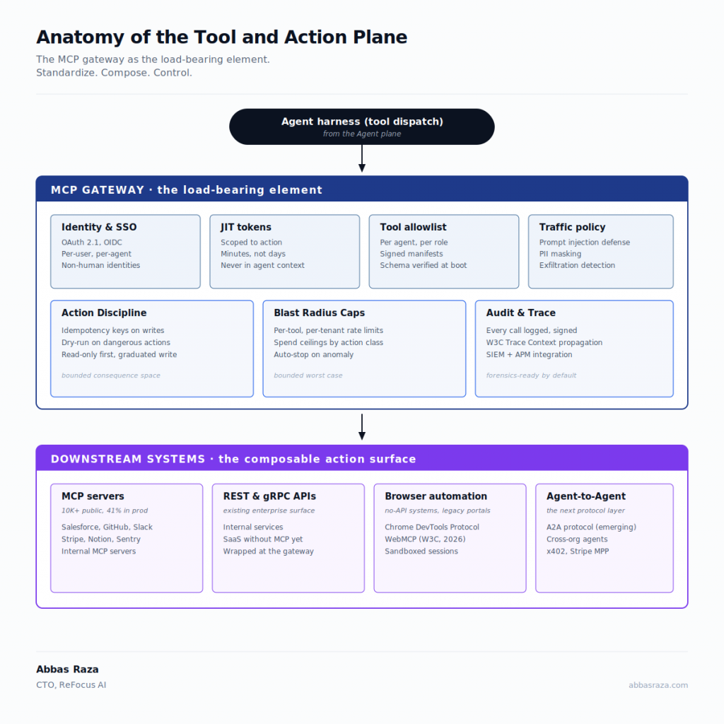
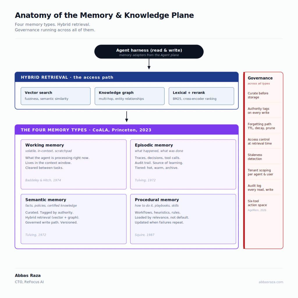
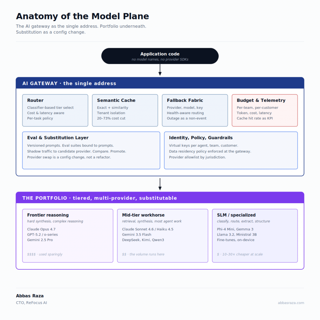
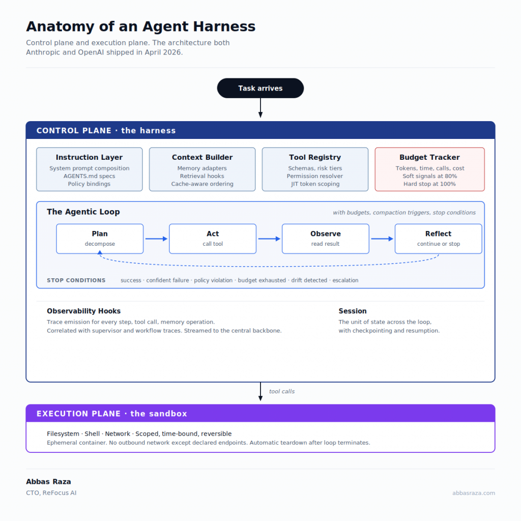
This is the sixth piece in a series on enterprise multi-agent architecture. The flagship laid out five planes and a Trust Fabric. The second piece went deep on the Agent plane. The third on the Model plane. The fourth on the Memory and Knowledge plane. The fifth on the Tool and Action plane. This piece goes inside the Orchestration and Experience plane and stays there. The Trust Fabric closes the series next.

The demo that stopped the meeting

A CIO at a Fortune 500 enterprise walks into a conference room in June 2026 for a demo his team has been building for four months. The team lead opens a laptop. On the screen is a clean, minimalist chat window. The team lead types a natural language request against a familiar workflow. The system takes ninety seconds to think. It responds with a paragraph of prose summarizing what it found and what it recommends. The prose is confident, well-written, and appears accurate.

The CIO reads it twice. He looks at the team lead.

“Where do I approve the actions?”

The team lead pauses. “The system just executes the recommended actions once you confirm in chat.”

“Where do I see what it’s about to do before it does it?”

Another pause. “You can ask it to explain.”

“Where do I see what it did last week? Last month?”

“You can search the chat history.”

“How do I hand this off to my head of procurement so she can review a specific decision?”

“You copy the chat link into an email.”

“How do I know which of the fourteen tool calls it made was the one that produced the wrong number?”

The team lead does not have an answer.

The CIO closes the laptop. The demo that impressed everyone in engineering does not survive first contact with the CIO’s actual questions. The chat is the interface. The chat is the entire interface. There is no plan view, no approval interface, no history that a human other than the original user can navigate, no accountability trail that anyone in the organization other than the team who built it can operate.

The team spends the next quarter rebuilding the experience layer. The model was fine. The harness was fine. The memory was fine. The tools were fine. The topology was under-thought. The interface was assumed rather than designed. This is where most enterprise agent deployments quietly fail in 2026.

The system had all of the intelligence and none of the discipline required to become a product.

The thesis

The Orchestration and Experience plane is where narrow agents compose into outcomes, and where those outcomes meet humans. It is where architecture becomes product.

Its core value is threefold. Topology fits the task, because the shape of the composition determines cost, latency, failure modes, and quality more than any individual model choice inside it. Cost and quality are architectural properties, not model properties, because the same models in different topologies produce different economics and different outcomes. The experience matches the nature of the work, because chat is a demo, delegation is a product, and enterprises that ship the demo without designing the delegation stop shipping shortly after.

Security lives here too, but as a facet of “topology fits the task” and “the experience matches the work.” Audit trails, blast-radius policies, human approval points, and observability are shape decisions on this plane, not add-ons. Everything you built on the four planes underneath (the reliable harness, the substitutable model portfolio, the typed memory stores, the disciplined action surface) either produces value on this plane or does not.

The rest of this piece defends each of the three properties and shows what they mean architecturally.

What changed in 2025 and 2026

Six inflection points reshaped what serious looks like on this plane.

Anthropic published its production orchestration architecture. The multi-agent research architecture behind Claude’s Research feature is now the most documented production orchestration pattern in the field. A lead agent (Opus 4) plans and coordinates. Three to five subagents (Sonnet 4) explore independent directions in parallel. Findings return through a shared memory store rather than through chat-style handoffs. A separate citation pass reconciles the synthesis. The internal evaluation showed a 90.2 percent improvement over single-agent Opus 4 on the research benchmark. The token cost was roughly 15 times a standard chat interaction. That trade curve is now the reference model that every other production team is measuring itself against.

The framework landscape consolidated. LangGraph became the production standard for stateful, auditable multi-agent workflows in early 2026, surpassing CrewAI in GitHub stars and dominant in enterprise references. Microsoft Agent Framework 1.0 reached general availability on April 3, 2026, unifying AutoGen and Semantic Kernel into one SDK with native MCP and A2A support, first-class C# alongside Python, and long-term Microsoft support commitments. OpenAI Agents SDK replaced the experimental Swarm as OpenAI’s production path. Google shipped ADK 1.0 for Java and Go early in the year. Anthropic’s Claude Agent SDK started drawing subscription usage from a separate monthly Agent SDK credit on June 15, 2026. The framework choice matters more than it did a year ago because the frameworks have crossed the durability threshold. It also matters less than the topology choice above it.

The topology mattered more than the model. Princeton’s HAL benchmark data showed that Claude Opus 4 scores 64.9 percent on GAIA inside one orchestration scaffold and 57.6 percent inside another. The gap between two orchestration choices on identical models is larger than the improvement between many frontier model releases. In practice, this means that the team that picked the right topology and the wrong model outperforms the team that picked the right model and the wrong topology.

The 2026 default became supervisor. Across current framework and pattern surveys, the supervisor pattern (a single orchestrator delegating to specialized subagents, one layer deep) is the production default. Anthropic’s research architecture uses it. LangGraph’s Supervisor template uses it. OpenAI Agents SDK handoffs converge on it. Claude Code subagents are architected around it. The reason is empirical: two layers of orchestration (orchestrator plus workers) handle the vast majority of enterprise cases, and adding more layers introduces coordination overhead that rarely pays for itself. The most common production mistake is stacking hierarchy before the complexity of the problem earns it.

The experience conversation broke open. For most of 2025, the discourse assumed chat was the interface. In the first half of 2026, that assumption collapsed under the weight of production experience. NN/g’s State of UX 2026 report named trust as the central AI design challenge and identified the “hybrid trap” (chat and GUI fighting for control) as one of the top adoption killers. The shift from conversational UI to delegative UI (users assigning goals rather than typing prompts) became the design consensus. Generative UI (interfaces drawn in real time from context rather than hard-coded per workflow) moved from research demo to shipping product. Gartner projected 40 percent of enterprise applications will embed task-specific agents by end of 2026, up from under 5 percent in 2025.

Human-on-the-loop replaced human-in-the-loop as the enterprise pattern. The 2024 discourse assumed a human would approve every consequential agent action. The 2026 practitioner consensus is that this scales poorly and produces approval fatigue that erodes the quality of oversight. The pattern that shipped is supervision: humans watch aggregates, intervene on exceptions, approve the classes of action that warrant it, and let the agent operate autonomously on the classes that do not. Microsoft Copilot Studio’s advanced approvals feature is the visible edge of this. The underlying discipline is picking approval points by risk tier, not by default.

Six shifts. One direction. The Orchestration and Experience plane went from an underdesigned afterthought eighteen months ago to a first-class engineering discipline with named frameworks, named patterns, and named consequences.

Topology fits the task

Six topologies dominate the 2026 production landscape. Each has a distinct cost profile, failure mode, and set of tasks it is appropriate for. Confusing them is the most common mistake I see.

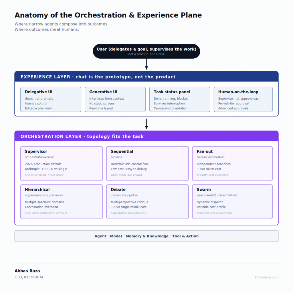
Supervisor (orchestrator-worker). A single orchestrator decomposes the task, delegates to specialized workers, and synthesizes the result. One layer deep. This is the 2026 production default. The Anthropic research architecture uses it. LangGraph’s Supervisor template uses it. It fits any workflow where a coordinator can plan and a set of specialists can execute in parallel or in sequence under coordination. Cost profile: dominated by the orchestrator’s growing context window as it accumulates worker results. Failure mode: the orchestrator becomes a bottleneck and a single point of context corruption.

Sequential (pipeline). A fixed chain of agents, each producing structured output that becomes the next agent’s input. Deterministic control flow. Low cost. Excellent debuggability. Fits workflows where the steps are known in advance and the branching is minimal: intake, extraction, classification, transformation, delivery. Cost profile: the sum of the individual agent calls, no orchestration overhead. Failure mode: rigidity. Any workflow variation outside the pipeline shape requires either a new pipeline or a wrapper.

Fan-out (parallel exploration). The orchestrator spawns N workers in parallel, each exploring an independent branch, and reconciles their outputs. This is the pattern behind the 90.2 percent Anthropic result. Cost profile: roughly 15 times a single-agent chat because you are running N context windows in parallel. Quality profile: excellent on breadth-first questions where the value of the outcome outweighs the token cost. Failure mode: false parallelism. If worker B’s task actually depends on worker A’s result, running them in parallel becomes expensive serial execution with extra overhead.

Hierarchical. Supervisors of supervisors. A top-level orchestrator delegates to mid-level supervisors who delegate to worker agents. Cost profile: high, because every layer adds coordination and context passing. Quality profile: worth it for genuinely complex workflows that span distinct domains, each with its own specialist supervisor. Failure mode: hierarchy added too early. Two layers handle most enterprise cases. Adding a third rarely pays for itself and introduces debugging pain that compounds.

Debate (consensus). Two or more agents produce independent analyses on the same input, and a judge model arbitrates. Microsoft Copilot Council is the reference public example, running GPT-5.4 and Claude in parallel with a judge model deciding between them. Cost profile: roughly 2.5 times a single-model call. Quality profile: valuable for high-stakes decisions where the cost of a wrong answer justifies the cost of running the analysis twice. Failure mode: cost creep. Once teams see the quality improvement they are tempted to apply the pattern everywhere, and the token cost stops being defensible.

Swarm (mesh). Peer agents hand off to each other directly, without a central orchestrator. Decentralized routing. Fits research tasks with dynamic dispatch, or coordination problems where the shape of the work is not knowable in advance. Cost profile: variable and hard to predict. Failure mode: coordination collapse. Without a supervisor to hold state, complex swarms can lose coherence in ways that are painful to debug.

The architectural discipline is picking the topology that fits the task, not the topology that fits the framework or the trend. Real production systems combine patterns. A common architecture: a supervisor at the top delegating to fan-out research workers, feeding into a sequential pipeline that produces a structured output, with a debate step gating the highest-stakes decisions and human-on-the-loop supervision above the entire flow. The patterns are composable. What matters is knowing which pattern operates at which layer, and why.

The most consequential decision on this plane is not which framework to use. It is which topology to build for.

Cost and quality are architectural properties

The empirical case for treating topology as architecture rather than as an implementation detail is now sharp enough to end the debate.

Anthropic’s published data on their research architecture is the most cited: multi-agent Opus 4 plus Sonnet 4 subagents beat single-agent Opus 4 by 90.2 percent on their internal research benchmark, at roughly 15 times the token cost. Token usage explains 80 percent of performance variance on browsing evaluations. This is not a model story. It is a topology story. Same models, different topology, radically different outcome.

The Princeton HAL benchmark result is the second reference point. Claude Opus 4 scores 64.9 percent on GAIA inside one orchestration scaffold and 57.6 percent inside another. That is a 30-percentage-point range on identical model weights, produced entirely by how the orchestration around the model is designed. Framework choice moves benchmark scores more than most frontier model releases. Topology choice moves them more than framework choice.

The practical implication for a CTO is that most of the leverage on cost and quality in an enterprise agent system lives on this plane, not on the Model plane. If you are optimizing your Model plane for cost and skipping the topology discussion, you are optimizing the wrong variable. If you are running debate patterns on low-stakes queries because your team thought the quality improvement was worth it, you are burning money that should be moving to fan-out patterns on the queries where breadth actually matters. Every topology has a right kind of task, and the cost profile is defensible only when the task fits.

Three operating rules that have earned their place:

Match the topology to the task, not the reverse. A supervisor pattern where a sequential pipeline would have worked is expensive misdirection. A debate pattern on a routine query is expensive theater. A fan-out pattern where a single agent could have answered in one call is expensive dilution. The starting question is what the task shape actually is: linear, branching, breadth-first, high-stakes, or research.

Measure the token cost of the topology, not just the model. The supervisor’s growing context window drives more of the unit economics than the worker calls do. The parallel branches in a fan-out drive more than the model per branch. Instrument this. Report cost per outcome, broken down by orchestration layer. The reports will tell you when the topology has grown beyond the value it produces.

Cap the layers. Two-layer orchestration (supervisor plus workers) handles the vast majority of enterprise cases. Three layers requires a specific justification. Four layers requires an unusual justification. The teams that ship reliably in 2026 tend to stop adding hierarchy before complexity accretes past the point of debuggability.

The framework and platform landscape

If the topology is the architecture, the framework is how you express the architecture. The 2026 framework landscape has consolidated around a small number of serious options, and picking between them is real work but secondary to picking the topology.

LangGraph is the production standard for stateful, auditable multi-agent workflows in 2026. It models agent workflows as directed graphs with typed state, checkpointing, and time-travel debugging. It is the framework I see most in enterprise references, in regulated industries, and in serious build-your-own orchestration efforts. Its main trade-off is a learning curve on the graph state model. Once teams internalize it, they rarely leave it.

Microsoft Agent Framework 1.0 shipped GA on April 3, 2026 as the unified successor to Semantic Kernel and AutoGen. Native MCP and A2A. First-class C# alongside Python. Tight Azure AI Foundry, Azure OpenAI, and Entra ID integration. If you are a Microsoft-shop enterprise, this is the framework that will get institutional support first.

OpenAI Agents SDK replaced Swarm as OpenAI’s production path. Clean handoff model, low learning curve, tight integration with OpenAI’s hosted tools. Trade-off: model-locked to OpenAI, no built-in checkpointing for long-running workflows, and the handoff pattern becomes unwieldy past eight or ten agents.

Google ADK shipped 1.0 for Java and Go alongside Python and TypeScript in early 2026. Strong Vertex AI integration and A2A Agent Cards for cross-team agent discovery.

Claude Agent SDK is Anthropic’s production SDK, integrated natively with MCP and the strongest ecosystem support for the “give the agent a computer” pattern. Started drawing a separate monthly Agent SDK credit on June 15, 2026.

CrewAI remains the fastest path from idea to working multi-agent prototype (roughly two to four hours). Trade-off: teams eventually outgrow the role-based abstraction for production workflows.

Above the framework layer sits the managed platform layer. If you need governance, identity, audit trails, and procurement-friendly licensing more than you need code-level control, the eight enterprise platforms that matter in 2026 are Microsoft Copilot Studio and Microsoft 365 Agents, AWS Bedrock AgentCore, Google Vertex AI Agent Builder, OpenAI Agent Platform, Salesforce Agentforce 360, ServiceNow AI Agents, IBM watsonx Orchestrate, and UiPath Agentic Automation. Most large programs I see run both layers: a managed platform for breadth (identity, audit, procurement) and a framework for the depth workflows where the topology genuinely matters. The build-vs-buy question is real, but the answer is usually both.

Roughly 28 percent of production multi-agent deployments in 2026 use custom orchestration rather than a framework. That number is neither an endorsement of custom nor a criticism of it. Custom is right when you have unusual observability or state requirements that no framework meets. Custom is wrong when you are avoiding a framework because the team has not internalized graph state or the handoff model. Learning the framework is cheaper than building the framework.

The experience matches the work

Everything above this section is orchestration. What follows is where the composed system meets humans. This is where most enterprise agent programs discover, uncomfortably, that they built the intelligence and did not design the delegation.

Chat is a prototype. Chat is where teams demonstrate that the intelligence works. Chat is where users learn what the system can do. Chat is not, for most enterprise workflows, the shape of the product.

The 2026 shift is from conversational UI to delegative UI. Conversational UI waits for the user to type a question and returns an answer. Delegative UI accepts a goal, shows the plan, executes the plan under supervision, and reports back with structured outputs the user can act on. The user is not a prompter. The user is a supervisor.

Four patterns anchor the discipline.

Delegative UI. Users assign goals rather than tasks. The interface captures intent in structured form (a form, a wizard, a bounded input flow) and lets the agent decompose the goal into tasks. The user does not type “Please compare these three vendors and produce a recommendation.” The user selects three vendors, picks a recommendation type, chooses a deadline, and delegates. The agent takes it from there. This shift is not cosmetic. It changes what the user thinks the system is: a colleague to whom work is delegated, not a chatbot to whom prompts are addressed.

Generative UI. Interfaces drawn in real time from context, rather than hard-coded per workflow. When the agent needs to show a comparison, the UI generates a comparison view. When the agent needs to show a timeline, the UI generates a timeline. When the agent needs to show a plan, the UI generates a plan view with the specific steps, the current status, and the expected completion. Jakob Nielsen’s framing, quoted throughout the 2026 design discourse, is that “the concept of a static interface where every user sees the same menu options, buttons, and layout, as determined by a UX designer in advance, is becoming obsolete.” The shift is happening now, unevenly, but the direction is clear.

Task status panel. A single view that shows what was done, what is running, what is blocked, and what is next. It survives interruption. A user who steps away for two hours can come back and see the state of the work without scrolling through conversation history. This is one of the highest-leverage patterns in the entire experience layer. Teams that build it report immediate adoption gains. Teams that assume chat history serves the same purpose learn otherwise the first time a user comes back to a long-running task and cannot find the state.

Human-on-the-loop supervision. The 2024 discourse assumed human-in-the-loop meant a human approves every consequential action. The 2026 practitioner consensus is that this scales poorly and produces approval fatigue that erodes the quality of oversight. The pattern that shipped is supervision: the human watches aggregates, intervenes on exceptions, approves the classes of action that warrant approval, and lets the agent operate autonomously on the classes that do not. Microsoft Copilot Studio’s advanced approvals feature is one visible implementation. The underlying discipline is picking approval points by risk tier, per action class, per tenant, with explicit thresholds. Not “the human approves everything” and not “the human approves nothing.” The right structured middle.

The failure mode on this layer has a name in the 2026 design literature: the hybrid trap. Conversational UI and agentic autonomy collide. Users are forced to choose which surface to trust. Chat says one thing, the GUI says another. Progress in chat does not update the GUI, and progress in the GUI does not update the chat. Adoption dies not because the intelligence failed but because the interface could not decide what it was.

The way out of the hybrid trap is to pick a shape. If the workflow is conversational, chat is the interface, and every other surface is a supporting detail behind it. If the workflow is delegative, delegative UI is the interface, and chat is a supporting affordance embedded in it. Do not build a system where chat and GUI compete for authority. Users cannot navigate that. Neither should you have to.

A worked example: the Risk Reassessment agent’s Orchestration and Experience plane

Recall the Risk Reassessment agent from the prior four pieces. Its job is to assemble a current view of a vendor’s risk profile by pulling SOC 2 history, security incident records, financial filings, and fresh external signals, then producing a structured risk score.

Its Orchestration and Experience plane looks like this.

At the orchestration layer, the agent runs a two-tier supervisor topology. A Renewal Supervisor coordinates the reassessment for a specific vendor. It delegates to four specialist workers running in fan-out: the risk data assembler, the financial signal analyzer, the security incident analyzer, and the external signals aggregator. Each worker has its own context window, its own tool allowlist through the MCP gateway, and its own model choice through the AI gateway (mostly Sonnet 4.6 for mid-tier work, occasionally escalating to Opus 4.7 when signal-conflict detection fires). The four workers return condensed structured findings to the supervisor through the shared memory plane (semantic memory for entities and relationships, episodic memory for prior reassessments of this vendor). The supervisor reconciles the findings, produces a structured risk score, and drafts the natural-language summary that flows into the Communication agent.

Total pattern: supervisor plus fan-out. Two layers. Roughly nine tool calls per reassessment. Blended token cost around six to eight times a single-agent chat, not fifteen, because the workers return condensed findings rather than long chat-style outputs. Median latency around ninety seconds. High tail-latency bounded because the workers run in parallel and the slowest branch caps the total.

At the experience layer, the interface is delegative. The procurement leader does not type prompts. She sees a queue of vendors due for reassessment. She can filter, sort, and select. She can delegate a reassessment with two clicks. The interface shows a plan view (what the supervisor plans to do, which workers it plans to spin up, which tools they will call, expected completion time). The plan is editable. If she wants to skip external signals for a specific vendor because they were just reviewed, she can. If she wants to force an escalation to Opus 4.7 for a high-stakes case, she can. The delegation captures her goal, the plan makes it operable, and the work proceeds.

A task status panel sits above the queue. It shows what was reassessed in the last week, what is running now, what is blocked (usually on human input or an external system outage), and what is scheduled for next. She can come back after a two-hour meeting and understand the state of the work in ten seconds. She does not scroll through chat history.

Human-on-the-loop is calibrated per action class. Low-risk reassessments (the vendor has been stable for four quarters, the risk score is unchanged) proceed autonomously and appear in the completed queue. Medium-risk reassessments (the risk score changed by more than one tier) route to her queue for review before any action. High-risk reassessments (a recommendation to terminate a contract) require explicit approval and route to her queue with the underlying evidence, the plan, and the specific action awaiting sign-off. Terminate-contract actions also require a second approval from the head of procurement. She never approves individual tool calls. She approves classes of outcomes. The advanced approval flow is calibrated on a risk tier that the system computes and presents.

The composition, the interface, and the supervision are not accidents. They are three architectural decisions made deliberately, with the assumption that the composed system needs to become a product before it becomes useful.

The 90-day move

If you are reading this and wondering where to begin, here is what I would do this quarter.

Name the topology explicitly. Whatever your agents are doing today, write down the topology. Supervisor. Sequential. Fan-out. Hierarchical. Debate. Swarm. If you cannot name it, you do not have one, and that is the first problem. Once it is named, ask whether the topology actually fits the task. If not, redesign to the shape that fits.
Pick the framework, or defend custom. LangGraph is the safest default for stateful production workflows in 2026. Microsoft Agent Framework 1.0 is the safest default on the Microsoft stack. If you are running custom orchestration, defend the decision explicitly with the specific requirements that no framework meets. If you cannot defend it, migrate.
Build the task status panel. What was done, what is running, what is blocked, what is next. In a single view. Above whatever else your interface does. This is one of the highest-leverage patterns in the entire experience layer, and most teams underbuild it.
Design the delegative flow. For each workflow your agents support, ask whether the user is prompting or delegating. If prompting, is that the right shape or an accident of history? Where the answer is delegation, build the delegative interface. Chat becomes a supporting affordance, not the surface.
Set human-on-the-loop by risk tier. Enumerate the classes of actions your agents can take. Assign each class an approval tier. Low-risk proceeds autonomously. Medium-risk queues for review. High-risk requires explicit approval, with the underlying evidence and plan surfaced together. Refuse to build a system where humans either approve everything or approve nothing. Both extremes are worse than the calibrated middle.

That is roughly a quarter of focused work for a small team. The payback shows up immediately as a reduction in the specific failure mode where the demo works and the product does not.

What this means

The flagship made the case that the model is not the product. The architecture is the product. Every deep dive since has refined that claim one layer at a time. The harness makes a model into a reliable agent. The model portfolio absorbs market churn. The typed memory stores make the system remember and forget deliberately. The disciplined action surface lets it operate on production systems. This plane is where all of that becomes a product a real business can operate.

Topology fits the task, because the shape of composition determines everything downstream. Cost and quality are architectural, because they live in the shape, not in the models. The experience matches the work, because chat is a demo and delegation is a product.

Name the topology. Pick the framework. Build the task status panel. Design delegation. Calibrate human-on-the-loop by risk tier. Watch the plan view, the approval flow, and the accountability trail as first-class citizens rather than afterthoughts. Assume that the system you are building will be operated by people who did not build it, and design accordingly.

The final piece in this series closes on the Trust Fabric: the cross-cutting set of controls (identity, policy, observability, evals, FinOps, human oversight, compliance) that turns the five planes into a system your business can put its name on.

The Tool and Action Plane

by AR, Posted on July 10, 2026

A deep dive on the Tool and Action plane. Why standardization changed the economics, why composability changed what agents can do, and why controllable autonomy is the discipline that turns capability into value.

This is the fifth piece in a series on enterprise multi-agent architecture. The flagship laid out five planes and a Trust Fabric. The second piece went deep on the Agent plane and the discipline of harness engineering. The third went deep on the Model plane and the AI gateway. The fourth went deep on the Memory and Knowledge plane and the discipline of curating before storage. This piece goes inside the Tool and Action plane and stays there.

The eight-application day

A senior analyst inside a Fortune 500 procurement organization begins her Monday morning by opening eight different systems in sequence. The vendor system-of-record. The SEC filings archive. The cyber-incident data source. The credit-rating provider. Two carrier portals with no API coverage. The sanctions screening service. The internal risk taxonomy tool. She spends the first two hours of her day copying identifiers between them, reconciling formats, and assembling a picture that no single system holds. By the time she has a coherent view of one vendor, she has performed roughly forty distinct operations across those eight systems.

She does this for a hundred and forty vendors a quarter. The pattern is familiar to anyone who has watched knowledge work happen in a large enterprise. AWS research on enterprise workflows reports that knowledge workers navigate eight to twelve different web applications during standard workflows. The work is not intellectually hard. It is operationally expensive. Every system has its own credentials, its own quirks, its own version of the same entities under slightly different names. The value is not in any one system. It is in the composition across systems, performed patiently, one identifier at a time.

This is the work the Tool and Action plane is built for. Not the reasoning, which lives in the Model plane. Not the recall, which lives in the Memory and Knowledge plane. Not the runtime discipline, which lives in the Agent plane. The Tool and Action plane is where autonomous software actually touches the systems, the data, and the workflows that carry the business. It is where an agent stops being an articulate observer and becomes software that operates.

Every plane in the reference architecture has one core purpose. The purpose of this plane is doing.

The thesis

The Tool and Action plane is the substrate where autonomous software actually does work in the world. Its core value is threefold: it standardizes how agents talk to systems, it makes capability composable across those systems, and it gives you controllable autonomy over what agents are allowed to do with that composed capability.

Standardization matters because without a protocol, every agent needs a bespoke adapter for every system, and the integration problem grows as the product of your agents and your tools. Composability matters because every real business outcome spans systems, and a plane that lets agents chain across them without custom code is what turns “an agent that can do one thing” into “an agent that can accomplish an outcome.” Controllable autonomy matters because doing work in the real world means writing to production systems, and the difference between an agent that produces value and an agent that produces incidents is whether the architecture lets you dial autonomy in and out, action by action.

Security lives inside controllable autonomy as one of its disciplines. So does safety. So does reliability. So does governance. A serious Tool and Action plane treats all four as facets of the same underlying idea: making autonomous action controllable at the architectural layer rather than hoping the agent gets it right.

The remainder of this piece defends each of the three properties and shows what they mean architecturally.

What changed in 2025 and 2026

Six inflection points reshaped what serious looks like on this plane.

MCP became the industry standard. Anthropic launched the Model Context Protocol in November 2024. In eighteen months it went from a company protocol to industry infrastructure. By Anthropic’s December 2025 ecosystem update, monthly SDK downloads across Python and TypeScript had passed 97 million, more than 10,000 active public MCP servers had shipped, and adoption spanned Claude, ChatGPT, Gemini, Microsoft Copilot, GitHub Copilot, Cursor, Windsurf, VS Code, and Zed on the client side. On the server side, Slack, GitHub, Google, Salesforce, Stripe, HubSpot, Shopify, Notion, Linear, Sentry, Figma, and Cloudflare had published official or community-maintained servers. The category consolidated fast because the underlying economic pressure was intense.

Governance moved out of Anthropic. In December 2025, Anthropic donated MCP to the Agentic AI Foundation (AAIF), a directed fund under the Linux Foundation, making the protocol vendor-neutral and community-governed. The precision matters: not just “donated to the Linux Foundation” in the way I loosely said in the flagship, but donated to AAIF under LF. AAIF is where the working-group governance actually lives.

The protocol matured. In March 2026, the maintainers published a 2026 roadmap organized around four priorities: transport evolution, agent communication, governance maturation, and enterprise readiness. In May 2026, the 2026-07-28 release candidate arrived. It is the largest revision since launch. A stateless core that scales on ordinary HTTP infrastructure. Extensions for server-rendered UIs (MCP Apps, SEP-1865) and long-running work (Tasks). Authorization aligned with OAuth 2.1 and OpenID Connect. W3C Trace Context propagation documented explicitly (SEP-414). A formal deprecation policy so the protocol can evolve without breaking what teams have already built.

Enterprise adoption crossed the production threshold. Stacklok’s 2026 State of MCP in Software report surveyed one hundred senior technical leaders and found 41 percent of software organizations in limited or broad production use of MCP servers, with 45 percent in the pure-software cohort. This is not experimentation. It is production.

Browser automation matured into a first-class action modality. Browser Use reached 89.1 percent on the WebVoyager benchmark across 586 web tasks. OpenAI’s Computer-Using Agent hit 87 percent on the same benchmark. Skyvern 2.0 reached 85.85 percent with a specialty in form-filling. Stagehand v3 shipped in February 2026 as a complete rewrite talking directly to Chrome DevTools Protocol, 44 percent faster than its predecessor. Google shipped an early preview of WebMCP in Chrome Canary in February 2026, developed jointly with Microsoft through the W3C. Browser action stopped being a fallback and started being an equal-class endpoint alongside MCP.

The security surface got named. OWASP published the Top 10 for Agentic Applications in December 2025, peer-reviewed by NIST, the Microsoft AI Red Team, and AWS. The taxonomy formalized what red teams had been finding all year: prompt injection through tool output (LLM01), supply chain vulnerabilities (LLM05), agent goal hijack (ASI01), and their cousins. Named threats produce named mitigations. The mitigations became architectural conventions on this plane.

Six shifts. One direction. The Tool and Action plane went from a wild frontier eighteen months ago to a governed infrastructure layer with named standards, named products, and named consequences. The economics of building agents that do useful work changed with them.

Standardization: from N times M to N plus M

Before MCP, integrating an agent with an enterprise system meant writing a bespoke adapter for every combination of model, provider, and tool. If you had N agents talking to M tools, you had roughly N times M integration pairs to maintain. Adding a new tool meant writing N adapters. Switching model providers meant rewriting M. Every organization I know that built agents in 2023 and 2024 hit a wall around the fifth or sixth tool because the maintenance cost of the adapter layer grew faster than the value the tools added.

MCP replaced that with a protocol on top of APIs. A single client can talk to any MCP server. A single server exposes tools to any MCP client. The N times M problem becomes N plus M. Every additional agent or tool adds one integration, not N or M.

This is the “USB-C for AI” framing that has become the standard shorthand. It is accurate. The protocol standardizes how an agent discovers what tools are available, how it calls them, how they authenticate (OAuth 2.1 as of the June 2025 spec), and how results flow back through a JSON-RPC base protocol. Server-rendered UIs (MCP Apps), long-running work (Tasks), and human-in-the-loop patterns (Sampling and Elicitation) round out the surface.

The reason to care about this at an executive level is not the protocol details. It is the strategic consequence. Standardization changes the economics of building agent-driven products. The unit cost of adding a new capability drops by roughly an order of magnitude when every tool speaks a common protocol. The unit cost of switching model providers drops by roughly the same amount, for the same reason I argued in the Model plane piece. The unit cost of onboarding a new team to build their own agents drops because the plumbing they inherit is already in place. Every one of these unit-cost drops compounds across quarters.

The strategic bet is durable because the industry converged. Anthropic launched it. OpenAI added native MCP support in early 2026. Google followed for Gemini. Microsoft integrated it across Copilot. AWS supports it in Bedrock. In mid-2026, building any new agent integration on a non-MCP protocol requires a specific reason. There will be edge cases, and the piece touches on them below, but the default is MCP and it will remain the default for the foreseeable future.

Composability: what the plane makes possible

Standardization is necessary but not sufficient. The reason it matters is that it enables composability, which is what actually creates value.

An agent that can call one tool well is an assistant. An agent that can chain across seven or eight tools in a single reasoning step is an operator. The move from assistant to operator is where the business value lives, because every real workflow spans systems.

Consider what “assemble a current view of vendor risk” actually requires. The vendor’s identifier in your system of record. Their SEC filings for the last four quarters. Any cyber incidents attributed to them or their subsidiaries in the last twelve months. Their credit rating and the trajectory of that rating. Whether they appear on any sanctions lists. The current status of their SOC 2 report. The commercial history you have with them. The list of customers currently exposed to them. No single system holds any of this. The value is entirely in the composition. A human analyst does this work in two hours, spread across eight applications. An agent operating over a composable Tool and Action plane does it in ninety seconds and returns a structured result.

The compounding effect is where the economics become interesting. Composability is not linear in the number of tools. It is combinatorial. Two composable tools give you two workflows. Ten composable tools give you thousands of possible chains. Twenty give you millions. This is why the enterprise agent market moved so fast in 2025 and 2026. Every new tool published to the ecosystem multiplied the possibility space for every agent that could reach it.

The architectural discipline that produces this compounding is that no tool integration should be written twice, and no agent should have to know the details of any specific tool implementation. Tools speak MCP. Agents call tools through the gateway. The gateway hides transport, authentication, and quirks. The agent reasons about capabilities, not about implementations. The plane’s job is to hide the mess so the reasoning above it can compose.

An adjacent capability worth naming here is Agent-to-Agent communication. Where MCP standardizes agent-to-tool, the emerging A2A protocol standardizes agent-to-agent. In an environment where agents from different organizations transact, coordinate, or subcontract to each other, the composability problem stops being about tools and starts being about agents themselves. The A2A specification is early in mid-2026. The design principles echo MCP: a JSON-RPC-based protocol, capability discovery, authentication, versioning. The gaps A2A fills include long-running task coordination and cross-organizational trust. Complementary technologies for agent payments (x402, Stripe MPP) are emerging alongside it. For a CTO, the pragmatic posture is to assume A2A will matter within eighteen months and to design the Tool and Action plane so a new protocol becomes another endpoint category behind the same gateway, not a rebuild.

Browser automation as a first-class action modality

Composability requires reaching every system where value lives. Some of those systems have APIs. Many do not, or their APIs cover only a fraction of what the UI exposes. In healthcare, EHR portals are the operational surface for scheduling, records, and prior authorization, and the API coverage is famously incomplete. In insurance, carrier portals are the substrate for quoting, endorsement, and renewals, and the API coverage varies dramatically by carrier. In finance, legacy systems and vendor portals are where a lot of the actual work happens, and the API surface can lag the UI by years.

If your agents are going to operate where the work actually happens, they will be driving browsers. This is not a hack. It is a permanent component of a serious agent architecture.

The 2026 capability picture is mature. Browser Use hits 89.1 percent on WebVoyager. OpenAI’s Computer-Using Agent hits 87 percent. Skyvern 2.0 hits 85.85 percent. Stagehand v3 is 44 percent faster than its predecessor. AWS Bedrock AgentCore ships Browser, Code Interpreter, and Identity services as first-class primitives.

WebMCP matters more than any of the benchmark numbers because it changes the trajectory. The Chrome Canary preview shipped in February 2026, developed by Google and Microsoft through the W3C. WebMCP is a protocol for structured AI agent interaction with websites: a Declarative API for HTML forms and standard page elements, and an Imperative API for dynamic JavaScript-driven interactions. The direction of travel is websites explicitly supporting agents rather than agents scraping websites. Once WebMCP is broadly adopted, the browser becomes a first-class action surface in exactly the way MCP made the tool ecosystem a first-class surface.

A legal dimension is worth naming, because it is coming for any CTO whose agents will drive third-party sites at scale. In late 2025, Amazon obtained a preliminary injunction against Perplexity’s Comet browser. The judge found Amazon likely to succeed on its claim that Perplexity violated the federal Computer Fraud and Abuse Act, drawing the distinction that matters: Comet accessed Amazon accounts “with the Amazon user’s permission, but without authorization by Amazon.” The Ninth Circuit stayed the injunction while the appeal proceeds. Perplexity filed a 96-page opening brief in April 2026 arguing the CFAA does not apply to an AI assistant running locally on a user’s device. The case is unresolved. The precedent forming is that a user’s permission to act on their behalf does not automatically override a website owner’s terms of service. If you are planning to build agents that drive third-party sites at scale, this is an issue for your general counsel, not just your architects.

Architecturally, browser action sits behind the same gateway as MCP tools. Sandboxed sessions with per-user identity. Consent flows for third-party access. Audit trails at the browser action level. Human-on-the-loop for anything transactional. The composability story treats browser action as an endpoint category alongside MCP servers, REST APIs, and A2A, not as a separate concern.

Controllable autonomy: the discipline that turns capability into value

Standardization and composability give you an agent that can, in principle, do a great deal. The next question is what it should be allowed to do, when, on whose authority, with what oversight, and with what recovery when it gets something wrong. This is the domain of controllable autonomy, and it is the third property of a serious Tool and Action plane.

Controllable autonomy is not about preventing the agent from acting. That framing is the mistake I see teams make when they first take the discipline seriously. The correct framing is that the plane provides architectural mechanisms for calibrating how much autonomy a given action is allowed to carry. The mechanisms are the same across security, safety, reliability, and governance because the underlying problem is the same: bound the consequence space of autonomous action so that the difference between “the agent got it right” and “the agent got it wrong” is not the difference between profit and catastrophe.

Six architectural disciplines make autonomy controllable. Every one of them belongs at the gateway or in the tool contract, not in each agent’s prompt.

Idempotency by default. Every write action requires an idempotency key. Repeated invocations with the same key produce the same result, not multiple side effects. This is not a nice-to-have. Agents retry. Harnesses recover from crashes. The same action is dispatched twice under normal operation. Without idempotency, controllable autonomy is impossible because the consequence space of a single decision is unbounded.

Dry-run mode on destructive actions. Any tool that mutates production state should also expose a mode that returns what would happen if the action ran, without executing it. The agent can preview. The harness can validate. The human oversight layer can review. In practice, this shifts the failure mode from “the agent did the wrong thing” to “the agent proposed the wrong thing and the gate caught it.” That is the correct place for that failure.

Read-only first, graduated write. New tools are exposed to agents in read-only mode first. Write access is added action-by-action, each one instrumented, reviewed, and gated on a run history that shows the agent uses it correctly. This is how you avoid the failure mode where an agent gets access to something it should not have because it was easier to grant the whole scope than to enumerate specific actions.

Just-in-time credentials. Credentials are minted at the moment of use, scoped to the specific action, and expire in minutes rather than days. The tokens themselves never enter the agent’s context window. The agent receives the results of an action, not the credentials that performed it. This is the single discipline that eliminates the largest category of credential-exposure risk, and it lives at the gateway.

Human-on-the-loop for high-consequence actions. The MCP specification’s Sampling and Elicitation features exist precisely for this. A destructive database migration, a large financial commitment, a customer-facing communication can pause for explicit human confirmation. The pattern is not “review the agent’s log at end of quarter.” It is “the agent stops and asks before it does something you would want to know about.”

Every action traced end to end. From the user’s request, through the agent’s reasoning, through the model call, through the gateway, through the tool, through downstream side effects, back to the user’s screen. W3C Trace Context propagation, now standardized in the 2026-07-28 RC, makes this possible with off-the-shelf tracing infrastructure. Teams that skip this discipline spend their time doing forensics after incidents. Teams that build it spend their time preventing them.

These six disciplines are the mechanics of controllable autonomy. They are what makes the difference between an architecture that lets you trust agents with reading a document today and posting a general ledger entry next quarter, and an architecture that never lets you cross that threshold safely.

The MCP gateway as the load-bearing element

Everything the plane needs to do (standardization, composability, controllable autonomy) has to happen somewhere. The where is the MCP gateway. It sits between your agents and every downstream MCP server, REST API, browser session, and A2A endpoint. Every tool call from every agent goes through it. Everything downstream trusts only the gateway, never the agent directly.

The gateway is where the plane’s three core properties become architecturally real. Standardization lives in the protocol translation the gateway performs across MCP servers, REST APIs wrapped as MCP tools, browser sessions, and A2A endpoints. Composability lives in the tool discovery and authentication the gateway provides so any agent can reach any allowed tool through a single interface. Controllable autonomy lives in the six disciplines the gateway enforces: identity and SSO for every call, JIT tokens scoped to specific actions, tool allowlists per agent and per role, action discipline (idempotency, dry-run, read-only first), blast radius caps per tool and per tenant, and end-to-end audit and trace.

The 2026 market for MCP gateways is real and consolidating. Arcade, Composio, Bifrost from Maxim AI, MCP Manager from Usercentrics, MintMCP, IBM Context Forge, Obot, and TrueFoundry are the names I see most in serious enterprise evaluations. The choice between them is real but secondary to the choice that comes first, which is to have a gateway at all. Direct agent-to-tool connections at any real scale in 2026 is an architectural anti-pattern, for the same reason direct application-to-database connections without a connection pool became an anti-pattern twenty years ago: it does not survive contact with production.

Where security fits

Security is one dimension of controllable autonomy, not the framing of the plane. But it is a dimension that has moved fast enough in the last six months that a serious piece has to name what has changed.

Between late 2025 and mid-2026, the threat surface got specific. OWASP published the Top 10 for Agentic Applications in December 2025. Check Point Research disclosed CVE-2025-59536 in Claude Code (CVSS 8.7), a configuration injection flaw via the Hooks mechanism. Cursor’s MCPoison and CurXecute vulnerabilities (CVE-2025-54136 and CVE-2025-54135) put tool poisoning on the map. CVE-2026-30615 in Windsurf and CVE-2026-27124 in FastMCP added prompt injection to RCE and OAuth misimplementation to the taxonomy. The postmark-mcp package became the first confirmed malicious MCP server in the wild by silently adding a BCC recipient to every email sent through it. In February 2026, the Sandworm_Mode campaign industrialized npm typosquatting against Claude Code, Cursor, and Windsurf. OX Security reported roughly 200,000 potentially vulnerable instances across the ecosystem and demonstrated that nine of eleven MCP registries accepted a proof-of-concept malicious package with no verification. In April 2026, CyberArk extended the tool poisoning family to full schema poisoning: attacks on parameter names, enum values, and response schemas, not just tool descriptions.

The pattern across these incidents is that autonomy plus a shared protocol expands the consequence space of a single compromised component, and that consequence space needs architectural containment. The containment already exists in the six disciplines of controllable autonomy above. JIT credentials cap the blast radius of a compromised server. Tool allowlists constrain which tools an agent can reach. Signed manifests and boot-time schema verification catch rug pulls and schema poisoning. End-to-end trace makes forensic recovery tractable when an incident does happen. The security architecture is not separate from the controllable autonomy architecture. It is the same architecture, viewed from a different angle.

The practical implication is that CTOs who put the gateway in place, adopt JIT credentials, enforce idempotency and dry-run at the tool contract, and instrument end-to-end trace have most of the security discipline they need to withstand the threat surface as it exists today. The specific threats will keep shifting. The architectural mitigations were valuable before the threats emerged and remain valuable as the threats evolve.

A worked example: the Risk Reassessment agent’s Tool and Action plane

Recall the Risk Reassessment agent from the harness, model, and memory pieces. Its job is to assemble a current view of a vendor’s risk profile by pulling SOC 2 history, security incident records, financial filings, and fresh external signals, then producing a structured risk score.

The composition it performs in one reassessment run is the value the plane creates.

The agent calls fourteen distinct tools across a typical run. Three are MCP servers built in-house: the vendor system-of-record, the SOC 2 archive, and the internal risk taxonomy service. Six are third-party MCP servers wrapped through commercial connectors: the SEC filings API, the cyber-incident data source, the vulnerability database, the news signal aggregator, the credit-rating provider, and the sanctions screening service. Three are traditional REST APIs that predate MCP and are exposed through a gateway-side adapter presenting them as MCP tools. Two are browser-automation flows against carrier portals that do not have API coverage, running in sandboxed Chrome sessions with per-user consent.

The composability point is not that any single one of these tools is impressive. It is that in ninety seconds the agent has assembled a coherent picture that a human analyst would spend two hours producing across the same fourteen systems. The reasoning above the plane is one third of the value. The composition the plane enables is the other two thirds.

Controllable autonomy shows up in the way the plane holds together at scale. The agent runs read-only against ten of the fourteen tools and never asks for more. Two tools have dry-run modes that the agent uses to preview any submission against a carrier portal before executing. Two tools require explicit human confirmation on final submission, which the harness surfaces through a workflow-native UI. Every call carries a JIT token scoped to the specific action, minted at the moment of use, valid for four minutes. Every action is traced end to end. When the schema drift detection on the news signal aggregator noticed a change in the tool description on a Tuesday morning, the aggregator was removed from the allowlist within an hour. No agent had used the changed version. The incident cost was zero. But the value the plane produced the day before, and the day after, was several thousand vendor reassessments performed at roughly one three-hundredth the analyst-hours the same work would require without composable, controllable, standardized tool access.

That is what one agent’s Tool and Action plane looks like when it works. The value is composability at scale, held together by controllable autonomy.

The 90-day move

If you are reading this and wondering where to begin, here is what I would do this quarter.

Stand up the MCP gateway. Pick one, install it, route every tool call in your agent codebase through it within four weeks. No exceptions. Everything goes through it. This is the keystone investment for this plane, the same way the AI gateway was for the Model plane.
Move to just-in-time credentials. Any tool that currently uses a long-lived token or API key gets rewired to mint tokens at the moment of use, scoped to the specific action, expiring in minutes. The agent never sees the credential.
Enforce idempotency and dry-run at the tool contract level. Every write action requires an idempotency key. Every destructive action exposes a dry-run mode. Build this into the tool definition, not into individual agent prompts.
Instrument audit and trace end to end. W3C Trace Context propagation through the gateway to downstream tools. Integration with your existing SIEM and APM. Every action tied back to the user, the agent, the model, and the intent.
Design browser action as a first-class modality. Sandboxed sessions, per-user identity, consent flows, human-on-the-loop for anything transactional. Do not treat it as a stopgap. It is a permanent component of the plane.

That is roughly a quarter of focused work for a small team. The payback shows up immediately as reduced integration cost, and compounds as your agents start composing across more tools and taking on higher-consequence actions that would have been unsafe without the discipline.

What this means

The flagship made the case that the model is not the product. The architecture is the product. The harness piece refined that claim into the runtime scaffolding that turns a model into a reliable agent. The model piece refined it into the substitutable, tiered portfolio that absorbs model market churn. The memory piece refined it into the four typed memory stores and the discipline of curating before storage. This piece refines it into the standardized, composable, controllable action surface where autonomous software meets your production systems.

You are not building a chatbot with tool calls. You are building a system that operates against your business, your customers, and your data, autonomously and at scale. The Tool and Action plane is the surface on which that operation happens. Standardization changes the economics of building it. Composability changes what it can do. Controllable autonomy changes what you can trust it with. The three properties are not independent. They are the same discipline expressed at different levels.

Stand up the MCP gateway. Move to just-in-time credentials. Enforce idempotency and dry-run at the tool contract. Instrument end-to-end trace. Design browser automation as a first-class modality. Watch A2A. Assume the threat surface will keep expanding, and design so that the same architecture that produced value yesterday continues to produce it as the surface evolves.

The sixth and next-to-last piece in this series goes deep on the Orchestration and Experience plane: how narrow agents compose into outcomes, why the topology of composition matters more than the individual agents, and why chat is the prototype for the interface rather than the interface itself. The Trust Fabric closes the series after that.

Curate Before You Store

by AR, Posted on June 20, 2026

A deep dive on the Memory and Knowledge plane. Why memory is where most agentic deployments quietly fail, and what to build instead.

This is the fourth piece in a series on enterprise multi-agent architecture. The flagship laid out five planes and a Trust Fabric. The second piece went deep on the Agent plane and the discipline of harness engineering. The third piece went deep on the Model plane and the AI gateway. This piece goes inside the Memory and Knowledge plane and stays there.

The eight weeks before anyone noticed

A category leader at a Fortune 500 procurement organization opens her queue on a Monday morning. The Renewal Supervisor has assembled a recommended action on a 2.3 million dollar enterprise contract: terminate the relationship, switch to a competing vendor. The justification is detailed. The Risk Reassessment agent cites the incumbent’s “ongoing security incident” and “deteriorating financial position per recent SEC filings.”

She approves. The vendor is notified. The migration kicks off.

Eight weeks later she learns the security incident was resolved fourteen months ago, and the SEC filings the agent referenced were from 2024, not “recent.” The incumbent’s reputation has been mishandled. They are entitled to compensation. She gets to face them across a table.

The model worked correctly. The harness ran exactly the loop it was designed to run. The tool calls returned exactly what the tools were configured to return. The failure happened in the memory plane: an episodic record that aged out of relevance without aging out of retrieval, a semantic memory entry that was never tagged with a temporal validity, a knowledge graph edge that pointed to financial data without a timestamp.

This is the failure mode that does not crash anything. The agent is confident. The reasoning is articulate. The action is wrong. By the time anyone notices, weeks have passed.

In the field, this is the category of failure that takes the longest to detect, costs the most to remediate, and burns the most trust between the system and the people who depend on it. It is also the category of failure that almost every production agent deployment ships with, because memory is the part of the architecture that most teams treat as an afterthought.

This piece is about why that has to change, and what changes it.

The thesis

Memory is where most agentic deployments quietly fail.

Production agents need four distinct memory types. They are not interchangeable. They differ in write authority, retention policy, retrieval pattern, and governance. Treating all four as a single vector database is the architectural equivalent of putting every table in your relational database into one denormalized blob and wondering why nothing scales.

A serious Memory and Knowledge plane has four properties. It is typed, because working, episodic, semantic, and procedural memory are not the same thing and should not be stored the same way. It is curated, because copying chaos into storage produces an agent that confidently cites whatever someone wrote in a Slack thread three quarters ago and forgot about. It is hybrid in retrieval, because vector search is necessary for unstructured fuzziness and embarrassingly bad at multi-hop reasoning about entities, relationships, and time. And it is governed, with authority tagging on every write, a forgetting path on every memory, and access controls enforced at retrieval time, not after.

Curate before you store. Build the forgetting path. Hybrid retrieval is the production answer. Memory is the long-term character of the system.

The remainder of this piece defends each of those claims.

What changed in 2025 and 2026

The Memory and Knowledge plane went from afterthought to first-class architectural concern in roughly eighteen months. A few inflection points are worth naming because they reshape what serious looks like.

The collapse of the “RAG is dead” narrative. Through late 2025, a meaningful share of the practitioner discourse argued that long context windows would make dedicated retrieval unnecessary. By May 2026, the VentureBeat Pulse enterprise survey data made the position untenable. Respondents identifying long-context-as-dominant-architecture collapsed from 15.5 percent in January to 3.5 percent in February before partially recovering to 6.7 percent in March. The enterprise market answered the question. Retrieval is not going away. It is becoming hybrid.

The CoALA framework as the consensus taxonomy. Sumers et al. at Princeton and CMU published Cognitive Architectures for Language Agents (arXiv:2309.02427) in 2023. By 2026 it is the canonical academic reference for the four memory types. Mem0, Letta (formerly MemGPT), LangChain, Zep, and LlamaIndex all use it as their taxonomy foundation. The cognitive science roots run deeper. Tulving distinguished episodic from semantic memory in 1972. Squire added procedural memory in 1987. Baddeley and Hitch formalized working memory in 1974. The taxonomy is not new. Its application as production architecture is.

Dedicated memory benchmarks. BEAM (Beyond a Million Tokens) emerged through 2026 as the industry-standard methodology for long-horizon memory evaluation. It scales to ten million tokens across one hundred procedurally generated multi-turn conversations and tests ten distinct memory dimensions including contradiction resolution, event ordering, instruction following across time, and preference tracking. The previous benchmark (LoCoMo) was found in a 2026 audit to contain score-corrupting errors in 6.4 percent of its ground-truth answer key. Memory evaluation finally has rigorous tooling.

Foundational research arriving. March 2026 brought the Governed Memory paper (arXiv:2603.17787), which formalized five structural failures of ungoverned multi-agent memory: memory silos, governance fragmentation, unstructured memories unusable by downstream systems, redundant context delivery, and silent quality degradation. The AgeMem framework (arXiv:2601.01885) defined a six-tool action space for memory operations: ADD, UPDATE, DELETE, RETRIEVE, SUMMARY, FILTER. The SSGM paper (arXiv:2603.11768) introduced a Stability and Safety Governed Memory framework. February’s “Rethinking Memory Mechanisms of Foundation Agents” survey (arXiv:2602.06052) consolidated three years of research into one reference. The field caught up to itself.

Microsoft GraphRAG reaching production maturity. Open-sourced in 2024, GraphRAG hit version 1.0 in 2026 with substantially better cost characteristics through the LazyGraphRAG optimization. Production deployments report up to 35 percent precision improvement over vector-only retrieval when knowledge graphs are integrated. Healthcare, finance, and legal sectors have been the early adopters, because each one has problems where the answer is a relationship rather than a document.

The Snowflake ontology result. Snowflake published internal research showing that adding an ontology layer to their agents produced a 20 percent improvement in answer accuracy and a 39 percent reduction in tool calls. The result is consequential because it is enterprise-scale, internally validated, and concrete. The ontology is entity identity mapping across systems, which is precisely the kind of structured knowledge that flat vector search cannot represent and that knowledge graphs handle natively.

Six inflection points. One direction. The Memory and Knowledge plane is now a designed system, not a database choice. Architectures that treated it as a database choice in 2024 are the architectures hitting the scale wall in 2026.

The four memory types

The CoALA taxonomy is the foundation. Production agents need four distinct memory types, designed deliberately.

Working memory. What the agent is processing right now. It lives in the context window and the active scratchpad. It is volatile by design. It clears between tasks. Working memory’s failure mode is overflow. As context fills, attention degrades, instructions buried in the middle get ignored, and the agent silently starts losing the thread. The harness piece covered the compaction patterns that mitigate this.

Episodic memory. What the agent has done and what happened. Traces, decisions, tool calls, outcomes. It is the audit trail. It is also the source of learning. Episodic memory needs to be tiered (hot, warm, archive) because not every interaction needs to be retrievable at the same latency forever. Its failure mode is the opposite of working memory: not overflow but staleness. An episodic record from fourteen months ago is sometimes the most relevant fact in the world and sometimes a hazard. The discipline is to know which.

Semantic memory. Facts and certified knowledge. The procurement playbook. The vendor commercial appetites. The customer coverage profile. Semantic memory is where most of the “curate before storage” discipline lives because it is the most consequential category and the easiest to pollute. Its failure mode is contamination: stale, low-quality, or hostile content makes its way in, and the agent confidently cites it forever.

Procedural memory. How to do things. Workflows. Heuristics. Playbooks. Procedural memory should be loaded by relevance to the current task, not by default, because loading too many playbooks consumes the context budget the working memory needs. Its failure mode is brittleness: a playbook that worked last quarter no longer matches the current process, and the agent applies it confidently anyway.

The most common failure I see is treating all four types as a single vector database. They differ in nearly every architectural dimension. Write authority differs (working memory writes on every step; semantic memory should require explicit curation). Retention policy differs (working memory clears immediately; episodic memory tiers; semantic memory is governed). Retrieval pattern differs (working memory is read at every reasoning step; semantic memory is read on retrieval; procedural memory is read on task initiation). Governance differs (working memory needs almost none; semantic memory needs the most). Designing all four with the same primitives produces a system in which the wrong content gets retrieved at the wrong time, repeatedly, and the agent appears confidently broken.

Hybrid retrieval as the production answer

Vector search is necessary. It is also not sufficient. The 2026 production consensus is hybrid retrieval, and the reason is mechanical.

Vector embeddings excel at semantic similarity. “Show me a passage about pricing changes” works well. They are embarrassingly bad at multi-hop structural reasoning. “Which suppliers serve competitors who recently entered our market?” requires traversing relationships across multiple entities. The vector database does not represent relationships. The knowledge graph does. The two technologies are not alternatives. They are complements.

The production pattern that has consolidated through 2026 has three components running in parallel, with the retrieval layer fusing the results.

Vector for fuzziness. Dense embeddings, semantic similarity, the standard RAG building block. Excellent for unstructured retrieval, document-oriented search, “find me content like this.” Pinecone, Weaviate, Milvus, Qdrant, ChromaDB are the established options. The standalone vector database category has been under pressure through 2026 as enterprises move toward hybrid, but the underlying capability remains essential.

Knowledge graph for structure. Property graphs that explicitly model entities and their relationships. Microsoft’s GraphRAG (open-sourced 2024, version 1.0 in 2026) and the LazyGraphRAG cost optimization that followed have brought knowledge graph adoption inside the cost envelope most enterprises can justify. The published precision improvement over vector-only retrieval runs up to 35 percent in domains where multi-hop reasoning matters, which is most enterprise domains. The Snowflake ontology result (20 percent accuracy improvement, 39 percent tool call reduction) is the cleanest single proof point.

Lexical search and reranking. BM25 keyword matching for exact-string requirements that semantic search misses. A cross-encoder reranker that re-scores the top candidates from vector and graph retrieval before they enter the prompt. Hybrid indexing with BM25 plus dense embeddings produces 15 to 30 percent precision improvements across enterprise deployments. The reranker is the unsung step. Most teams skip it and pay for it later.

The architectural move is to run all three in parallel and fuse the results. Reciprocal Rank Fusion (RRF) is the standard merge algorithm and works well enough for most production traffic. The retrieval layer’s job is not to pick the right method per query. It is to run the right methods in parallel and rank what comes back. The agent then reasons over a curated, ranked, multi-source result set.

This is what serious in 2026 looks like. Not “RAG with a vector database.” Not “agentic memory replaces retrieval.” Hybrid retrieval over four typed memory stores, with the agent orchestrating both.

The taxonomy of memory failures

Six failure modes I have seen consistently across deployments, my own and others’:

Memory contamination. Stale, low-quality, or hostile content makes its way into semantic or episodic memory and the agent confidently cites it forever. The 2026 Gamage study of 4,416 trials across six conversation depths quantified the downstream effect: constraint compliance dropped from 73 percent at turn 5 to 33 percent at turn 16 without memory mitigation. Halfway through a task, the agent is violating its own instructions twice as often as it was at the start. It does not know this is happening. It keeps running confidently.

Stale memory poisoning. A specific case of contamination worth naming separately. A tool returns data that was correct at retrieval time but becomes stale across the session. The agent integrates the data as fact, and every subsequent reasoning step builds on a premise that has moved underneath it. The opening scenario was a textbook case. The fix requires temporal validity on stored memories and active staleness detection at retrieval, not passive time-based decay alone.

Confident wrong citation. The agent retrieves the wrong document or the wrong record and cites it persuasively. The retrieval looks fine on standard metrics like NDCG or recall at k. The cited content semantically matched the query. It just was not the right content. This is the failure mode in regulated domains: clinical trial data from 2022 retrieved for a query that needed the 2025 safety profile, executive compensation documents retrieved because they semantically matched a benefits question.

Access control leakage. The retrieval layer returns results that semantically match the query without considering whether the requesting user is authorized to see them. Industry analysis suggests this risk is present in at least 73 percent of production RAG implementations. The most common incident: employees receiving context from board minutes or executive compensation documents because the retrieval layer ignored the access controls that the underlying document management system enforced. The fix is retrieval-native access control: permission predicates embedded in the retrieval query, not applied as a post-filter.

Cross-session identity drift. The agent loses track of who the user is across sessions. A returning customer is treated as new. A canceled vendor is treated as active. Identity in memory is a hard, open problem in 2026, and the Mem0 State of AI Agent Memory report names it as one of the three hardest unresolved problems alongside temporal abstraction at scale and memory staleness.

The five governance failures from the Governed Memory paper. Memory silos (each agent maintains its own memory, none can read another’s). Governance fragmentation (no consistent policy on what gets stored, who can read, when memory is forgotten). Unstructured memories unusable by downstream systems (stored in formats that subsequent agents cannot consume). Redundant context delivery (the same content retrieved repeatedly, paying for it every time). Silent quality degradation (memory quality decays without any signal that it is decaying).

These six are not exotic. They are the ordinary ways memory breaks. A serious memory engineering practice means you have explicit detection and mitigation for each.

Curate before you store

The discipline that prevents most of the failures above is the discipline of curating before storage.

The principle is simple to state and hard to maintain. The write path to semantic memory is governed. Not every document, not every tool response, not every agent observation flows into long-term memory by default. Each candidate is tagged for authority before storage. Each is tagged for temporal validity. Each is tagged for the tenant or scope that owns it. Each is reviewed against the access controls of its source. What enters semantic memory is what your organization considers true, current, and authorized to share with the agent.

Three operational rules:

Tag by authority level. Policy and Standard go in. Opinion and draft do not. The same source system can produce content at different authority levels. The procurement policy database is authoritative. A Slack thread debating the policy is not, even if both technically describe the policy. The agent should know the difference, which means the memory plane should know the difference, which means the write path should tag the difference.

Build the forgetting path. Most teams forget to. Every memory should have a temporal validity, a freshness signal, and an explicit prune mechanism. TTL on episodic records. Decay on low-relevance content. Active staleness detection on high-relevance content (the open problem). The forgetting path is not a cleanup job that runs once a quarter. It is a primary memory operation that fires continuously.

Use a structured action space. The AgeMem framework defines six memory operations: ADD inserts new entries, UPDATE modifies existing ones, DELETE actively prunes stale or redundant knowledge, RETRIEVE pulls relevant content, SUMMARY consolidates, and FILTER manages the boundaries of working context. The architectural move is to treat memory operations as a first-class API, not as a side effect of model inference. Every write is intentional. Every delete is intentional. Every update preserves audit history.

The deepest version of this principle, which I have come to repeat to every new engineer on the team: do not copy chaos. Connect to truth. When you ingest enterprise content into your memory plane, you are choosing what your agents will believe. Choose deliberately.

A worked example: the Risk Reassessment agent’s memory plane

Recall the Risk Reassessment agent from the harness and model pieces. Its job is to assemble a current view of a vendor’s risk profile by pulling SOC 2 history, security incident records, financial filings, and fresh external signals, then producing a structured risk score.

Here is what its memory plane looks like.

Its working memory holds the current task: this vendor, this renewal window, this risk reassessment in flight. It is the context window plus an active scratchpad that the harness manages. It clears when the task completes.

Its episodic memory holds the agent’s prior risk reassessments on this vendor, tiered by recency. The last six months sit in a hot tier with sub-second retrieval. The next two years sit in a warm tier. Older history sits in archive and is retrievable on explicit request. Every reassessment includes the date, the sources cited, the score produced, and the human review outcome. When the agent runs against a vendor it has reassessed before, episodic memory is what makes the new reassessment incremental rather than from scratch.

Its semantic memory holds the certified facts. The organization’s risk taxonomy. The vendor risk policy. The standard set of carriers and their commercial appetites. The supplier ontology that maps entity identity across procurement, legal, finance, and security systems. Every entry has an authority tag. Policy and Standard documents are present. Drafts and proposals are not. Every entry has a temporal validity. SOC 2 reports older than fifteen months trigger a staleness flag at retrieval.

Its procedural memory holds the playbooks for the reassessment workflow itself. The standard sequence of checks. The escalation criteria. The diagnostic patterns for unusual signal combinations. The agent loads only the playbook relevant to the current case, not all of them. When the playbook fails (the human reviewer overrides the recommendation, or the recommendation later proves wrong) the failure is logged and the playbook is updated for future runs. The harness piece called this the eval flywheel. The memory plane is where it lives.

The retrieval layer runs three methods in parallel. Vector search finds semantically similar content (passages about similar incident patterns). The knowledge graph traverses entity relationships (this vendor’s parent companies, subsidiaries, suppliers, and the customers exposed to them). Lexical search and reranking handle exact-match requirements (a specific CVE identifier, a specific regulatory citation). The agent reasons over a fused, ranked result set.

Governance runs across all four memory types. Authority tagging on every write to semantic memory. TTL on every episodic entry. Access control predicates embedded in every retrieval query, scoped to the calling agent’s identity. Audit logs on every read and every write. Tenant scoping on shared infrastructure so that one customer’s memory cannot leak into another’s reasoning.

The Snowflake-style productivity gain shows up across a quarter of operation. The structured ontology reduces redundant tool calls by roughly a third. The episodic memory of prior reassessments lets the agent skip work that has already been done. Hybrid retrieval lifts the precision of evidence the agent reasons over. The combination produces answers that the procurement leader can act on without spending eight weeks wondering whether the agent was right.

That is what one agent’s memory plane looks like in production. Multiply across an environment of dozens of agents and you start to see why the Memory and Knowledge plane, properly designed, is the difference between a system that compounds in usefulness over quarters and a system that degrades silently into expensive nonsense.

What I would do differently

The lessons below are the ones I paid for. I share them in the hope that they cost you less.

I underbuilt the forgetting path for too long. We had episodic memory accumulating for a year before we built a real pruning strategy. By the time we built it, retrieval quality on the older content was visibly degrading, and we did not have a clean way to know which entries were still relevant. Build the forgetting path before you need it. TTL on every entry. Decay on low-relevance content. Active staleness detection on high-relevance content from day one.

I treated all memory as one vector database. It was easier. It was also wrong. The four memory types differ in nearly every architectural dimension, and conflating them produces a system in which the wrong content gets retrieved at the wrong time. Type your memory from the start. Storing it in different substrates is fine. Pretending it is one thing is not.

I shipped without staleness detection. Our early agents retrieved content based on semantic similarity and recency, without any explicit signal of whether the content was still valid. The first time a confidently-wrong recommendation cost a customer relationship, we built temporal validity into the schema. It should have been there from the start.

I underestimated the access control problem. Retrieval-native access control was an afterthought in our early architecture. We patched it later by applying user-permission filters as a post-retrieval step. That works until the day a permission-restricted document leaks into an agent’s reasoning through the embeddings, even if it does not appear in the final answer. The fix is permission predicates embedded in the retrieval query itself, not post-filters. The earlier this is built, the less expensive it is.

I did not invest in the knowledge graph soon enough. We were vector-only for the first two years. The agents could handle “find me content like this” perfectly well. They could not handle “which suppliers serve competitors who recently entered our market.” When we finally built the knowledge graph layer, several entire categories of agent failure disappeared. If I had to start over, the knowledge graph would be in the architecture from week one, even with a small initial entity set.

The 90-day move

If you are reading this and wondering where to begin, here is what I would do this quarter.

Stand up the registry of memory writes. Every write to semantic or episodic memory, by any agent, gets logged with the source, the authority tag, the temporal validity, the tenant scope, and the writing agent’s identity. This is the equivalent of the agent registry from the harness piece, applied to memory. Build it on day one.
Instrument staleness. Add a freshness signal to every memory entry. Set thresholds per memory type and per content category. Surface staleness on every retrieval. Build a dashboard that shows the staleness distribution across your memory plane.
Add a knowledge graph for entity-relationship reasoning. Start small. The supplier ontology, the customer hierarchy, the product taxonomy. Use Microsoft GraphRAG or one of the established commercial options. The cost of starting is lower than it was a year ago. The cost of not starting is higher than it was a year ago.
Validate retrieval against access controls. Embed permission predicates in the retrieval query, not as post-filters. Test that restricted documents cannot enter the reasoning stream of an agent acting on behalf of a user without the relevant permissions.
Build the forgetting path. TTL on every episodic entry. Decay on low-relevance content. Active staleness detection on high-relevance content. Treat memory operations as a six-tool action space (ADD, UPDATE, DELETE, RETRIEVE, SUMMARY, FILTER) with audit on each operation.

That is roughly a quarter of focused work for a small team. The payback shows up immediately as a reduction in confidently-wrong answers, and compounds over quarters as the system’s long-term character becomes something the business can rely on.

What this means

The flagship made the case that the model is not the product. The architecture is the product. The harness piece refined that claim into the runtime scaffolding that makes a model into a reliable agent. The model piece refined it into the substitutable, tiered, gateway-served portfolio that absorbs model market churn. This piece refines it one layer further, into the memory plane that gives the system its long-term character.

You are not building chat. You are building an agent that has to remember the right things, forget the right things, retrieve the right things, and refuse to confidently cite the wrong things. The system’s character lives here. So does its credibility.

Build the four memory types. Run hybrid retrieval. Curate before storage. Build the forgetting path. Govern access at retrieval, not after. Tag authority on every write. Treat memory operations as a first-class API.

The next and final piece in this series goes deep on the Trust Fabric: the cross-cutting set of controls (identity, policy, observability, evals, FinOps, human oversight, compliance) that turns the five planes into a system the business can put its name on.

The Model Is a Portfolio, Not a Pick

by AR, Posted on June 14, 2026

A deep dive on the Model plane. Why frontier model choice is the wrong question, what an AI gateway actually does, and how to design for a market that is commoditizing in real time.

This is the third piece in a series on enterprise multi-agent architecture. The flagship laid out five planes and a Trust Fabric. The second piece went deep on the Agent plane and the discipline of harness engineering. This piece goes inside the Model plane and stays there.

The model market broke this week

Last Wednesday, the Wall Street Journal reported that OpenAI is in active discussions to lower its token prices substantially. The reason is not generosity. Anthropic just closed a sixty-five billion dollar Series H at a valuation approaching one trillion dollars, ahead of an IPO filing. Google cut its premium AI Ultra tier from $250 to $200 at I/O on May 19, added a new $100 entry point, and positioned Gemini 3.5 Flash at roughly seventy percent below frontier pricing. Chinese models from DeepSeek, Kimi, and Zhipu are running the same enterprise workloads at roughly one-ninth the cost of US frontier providers. The widely-cited comparison: a workload that costs $4,811 on Anthropic Claude runs for $544 on Zhipu’s GLM.

The model layer is commoditizing in real time. By the time you finish this essay, some of the prices in the paragraph above may already be wrong. The architectural lesson is not which provider to bet on next. It is to stop betting at all.

I have been saying for three years that the model is not the product. The architecture is the product. That claim has aged well. What it requires of you, as a CTO or architect, is a Model plane that does not depend on any one provider being the right answer for any one task at any one moment. You need a portfolio. You need a gateway. You need substitution as a config change. The teams that have this already are spending an afternoon doing what their competitors will spend a quarter doing. The teams that do not have it yet are about to learn the most expensive lesson of 2026.

This piece is the architecture for that lesson.

The thesis

You are not picking a model. You are building a portfolio.

The instinct of most engineering teams is to pick a frontier model the way you would pick a database. Choose carefully, integrate deeply, optimize over years. That instinct was always wrong, and the events of the last six months have made it actively dangerous.

A serious Model plane has four properties. It is multi-provider by default, because any single provider is one outage, one pricing change, one quality regression, or one geopolitical shift away from breaking your business. It is tiered, because the cost gap between a small specialized model and a frontier reasoning model is now between ten and thirty times for tasks where both perform comparably. It is routed, because the right model for classifying a customer message is not the right model for synthesizing a six-source analysis. And it is cached, because in real-world workloads a meaningful share of requests are semantically similar, and you should not pay for the same answer twice.

The mechanical realization of all four properties is an AI gateway sitting between your application code and every model provider. Everything below is what that means in detail.

What changed in 2025 and 2026

A quick walk through the events that have reshaped the Model plane in the last twelve months, because the events are the argument.

January 2026: DeepSeek-R1. A Chinese lab released a reasoning model that matched GPT-4-class performance at roughly one one-hundredth of the inference cost. Within two weeks, every CTO with a single-provider strategy was being asked the same question by their board: how fast can we switch? The teams that could answer “a config change, this afternoon” had built the right architecture. The teams that had to answer “a quarter, maybe two” started a project they could not avoid.

March 2, 2026: Anthropic outage. A multi-hour incident took down Claude.ai, the developer console, and Claude Code worldwide. The Wall Street Journal followed up in April with reporting that Anthropic’s API uptime over the prior ninety days sat at 98.95 percent. The cloud benchmark for serious infrastructure is 99.99 percent. The gap between those two numbers is roughly eight hours of downtime per year versus roughly four days. For an enterprise running production agents on a single provider, that gap is not a footnote. It is a quarterly board question.

March 31, 2026: Claude Code source map leak. A missing entry in Anthropic’s .npmignore shipped roughly five hundred thousand lines of TypeScript across nineteen hundred files. The community confirmed what practitioners suspected: building reliable AI agents is primarily an orchestration engineering problem, not a model capability problem. I covered this in detail in the harness piece. It is relevant here because every architectural lesson it teaches points downstream into the Model plane.

May 19, 2026: Google I/O pricing reset. Google cut AI Ultra from $250 to $200, introduced a $100 tier, and positioned Gemini 3.5 Flash at roughly seventy percent below rival frontier token pricing. Pichai claimed enterprises could save over one billion dollars in annual costs by migrating eighty percent of workloads to Gemini. The number is marketing. The directional signal is real.

June 2026: OpenAI considers price cuts. The Wall Street Journal report last week documented active internal discussions at OpenAI about lowering token prices significantly. This is what the bottom of a price discovery process looks like. The frontier providers are now competing on price, which means the frontier itself is becoming a commodity input.

Throughout: the LiteLLM supply chain attack. A widely-used open-source gateway library was briefly compromised through credential theft. PyPI later reported that the affected versions were downloaded over 119,000 times during the attack window. The lesson is not that LiteLLM is uniquely risky. The lesson is that the gateway layer is now critical infrastructure, which means it is also a high-value target. Owning your own deployment boundary matters more than it did a year ago.

Six events. One direction. The model market is moving from a small number of expensive frontier options toward a large number of substitutable options at sharply diverging price points. Your architecture has to absorb that motion without your application code noticing.

The AI gateway

The AI gateway is the architectural answer to all of the above. It sits between your application code and every model provider you call. Your application calls one address. The gateway routes, caches, falls back, enforces budgets, emits telemetry, and abstracts the differences between providers.

The 2026 gateway landscape has consolidated around roughly half a dozen serious choices: LiteLLM Proxy, Portkey, Cloudflare AI Gateway, Vercel AI Gateway, Kong AI Gateway, OpenRouter, and a handful of newer entrants like Bifrost and Helicone. Each makes different trade-offs on performance overhead, self-hosting flexibility, governance depth, and provider coverage. The choice between them is real but secondary to the choice that comes first, which is to have a gateway at all.

The non-negotiables of a serious gateway:

One endpoint to your application. Your code calls a single address. It does not know about provider SDKs. It does not contain model name string literals. It does not have retry-on-provider-error logic. If a model identifier appears as a string literal anywhere outside your gateway configuration, you have built the wrong abstraction.

Per-team, per-customer, per-agent virtual keys. Each consumer of the gateway gets a scoped key with its own budget, its own provider allowlist, and its own audit trail. When a runaway agent generates a five-figure invoice, you should be able to identify which agent, which workflow, and which customer in under a minute.

Health-aware fallback at three levels. Provider-level (Anthropic is degraded, route to OpenAI), model-level (Opus 4.7 is slow today, route to Sonnet 4.6), and key-level (this customer’s quota is exhausted, route to a backup key). The fallback chain is configurable per request class.

Semantic caching as a first-class component. Not bolted on. AWS-published research on 63,796 real production queries showed that at optimal similarity thresholds, semantic caching delivered an eighty-six percent cost reduction and an eighty-eight percent latency improvement on cached responses, with cache hit rates above ninety percent maintaining ninety-one percent response accuracy. Production deployments routinely report twenty to seventy-three percent token cost reduction depending on workload repetition. Cache hit rate should be a first-class KPI on your engineering dashboard. Most teams do not measure it.

Eval suites bound to prompts, not to models. When a new provider releases a stronger or cheaper option, you should be able to run your evals against it, in shadow, before any production traffic moves. If your evals only work with one provider’s API shape, you have an eval problem and a substitution problem at the same time.

The deeper play is to design the entire gateway for substitution. Provider swap should be a configuration change followed by a shadow comparison followed by a graduated promotion. The teams that get this right will spend an afternoon doing what their competitors spend a quarter doing.

Tiering: the portfolio inside the portfolio

Multi-provider is half the picture. The other half is tiering inside the portfolio.

There are three tiers, and almost every production workload uses all three.

Frontier reasoning. Claude Opus 4.7, GPT-5.2 and the o-series, Gemini 2.5 Pro. Used sparingly, for the hardest synthesis, the most consequential decisions, the work where reasoning quality is the bottleneck. Even inside one provider’s lineup, the price spread between frontier and mid-tier is now severe. Anthropic’s Claude Haiku 4.5 is roughly eighteen times cheaper than Claude Opus 4.7 as of April 2026 pricing. That eighteen-times spread inside one vendor’s catalog is the tiering argument in numerical form.

Mid-tier workhorse. Claude Sonnet 4.6, Claude Haiku 4.5, Gemini 3.5 Flash, the better open-weights mid-tier options. This is where most of the volume runs. Retrieval-shaped work. Synthesis with bounded context. Routine agent steps. Most production reasoning lives here.

SLM and specialized. Phi-4 Mini, Gemma 3, Llama 3.2 1B and 3B, Mistral Ministral 3B, Qwen3. Used for classification, routing, structured extraction, format conversion, intent detection, content moderation. Often fine-tuned on your data and hosted on your infrastructure. The economics are striking. Running a private SLM endpoint for ten thousand daily queries typically costs $500 to $2,000 per month. The equivalent workload on frontier APIs runs $5,000 to $50,000 per month, a five-to-twenty-times gap that widens with volume.

The architectural move is to route by task complexity, not by team preference. A classifier-based router sits in front of the gateway and decides, per request, which tier and which provider gets the call. The classifier itself is usually a small fast model. Cost-aware routing, latency-aware routing, and quality-aware routing are all variations on this theme. The teams that route well report production cost reductions in the forty to seventy percent range without measurable quality regression. The teams that route everything to the frontier are paying for capability they do not need on most of their traffic.

A pattern worth naming that is starting to spread through 2026: speculative decoding. A small fast model drafts a sequence of tokens. A frontier model verifies and either accepts or corrects. The net effect is roughly two to three times speedup on inference with no measurable quality loss. The harness layer makes this trivial to implement once the gateway is in place. The model layer’s job is to make both models available behind one address.

The Chinese model surge and what to do about it

Most Western CTOs have not seriously evaluated DeepSeek, Kimi, or Zhipu yet. The reasons are partly geopolitical caution, partly data residency concern, partly the simple inertia of an existing vendor relationship. Those reasons are not wrong. They are also not sufficient as an architectural posture.

The numbers are stark. DeepSeek-R1 matches GPT-4-class reasoning at roughly one-hundredth the inference cost. Zhipu’s GLM handles workloads at roughly one-ninth the cost of equivalent Anthropic Claude calls. Qwen3 is competitive with Western mid-tier models on most benchmarks. Kimi handles long-context tasks at price points that no Western provider can match today. The capability is real. The price arbitrage is real. And the gap is wide enough that boards have started asking about it directly.

The honest architectural answer is not to migrate workloads wholesale to Chinese providers. The honest answer is also not to ignore them. The answer is the same answer the gateway gives to every provider question: keep your options open.

In practice, this means three things.

Make Chinese model providers available behind your gateway. Not necessarily for production traffic today. For evaluation. For benchmark runs. For workloads where data residency and regulatory constraints do not apply. The gateway abstraction makes the cost of having them available roughly zero. The cost of not having them available, when your board asks why a competitor’s unit economics look better than yours, is high.

Set provider allowlists per workload sensitivity tier. A jurisdiction-aware policy at the gateway level lets you route customer-data-bearing traffic to providers with the right contractual and residency posture, while routing non-sensitive evaluation traffic anywhere. The Trust Fabric piece will cover this in more detail. The Model plane’s job is to make the policy enforceable.

Treat the geopolitical landscape as a variable, not a constant. Export controls shift. Data residency rules shift. Provider availability shifts. Architectures that depend on a constant geopolitical landscape are not architectures, they are bets. A gateway with a multi-provider portfolio is the only architectural posture that survives the next four years intact regardless of how the politics actually go.

The summary version, for the CEO who reads only this paragraph: you do not need to use Chinese models. You need to be able to use them if and when you decide to. That capability is what the gateway gives you.

Semantic caching: the unsung component

The cheapest call is the one you do not make.

Semantic caching is the practice of recognizing that two requests with different wording have the same meaning, and serving the cached response for both. It is not exact-match caching, which is what most teams build first and which catches roughly nothing in real production traffic. It is similarity-based caching using vector embeddings, with a configurable similarity threshold per request class.

The production numbers are excellent. The AWS research I cited above (63,796 real chatbot queries) is the cleanest published result. Eighty-six percent cost reduction. Eighty-eight percent latency improvement. Cache hit rates above ninety percent at high similarity thresholds, with response accuracy still above ninety-one percent. Academic research on the GPT Semantic Cache implementation reported hit rates between 61.6 and 68.8 percent across query categories with positive hit accuracy exceeding ninety-seven percent. Most production teams running this pattern report twenty to seventy-three percent token cost reduction depending on how repetitive their workload is.

A few design rules that have earned their place:

Dual-layer caching. Exact-match hash first, then semantic similarity. Exact matches are free to look up and produce no false positives. Semantic matches are slightly more expensive and require a confidence threshold. Run them in that order.

Tenant-scoped cache isolation. Cache entries scoped per customer, per agent, or per virtual key. A response cached for one tenant should never be served to another. The gateway is where this isolation lives.

Per-class similarity thresholds. A factual question can serve a cached response at a moderate similarity threshold. A code generation request needs a much higher threshold or no cache at all. The threshold is a per-route configuration, not a global constant.

Cache hit rate as a first-class KPI. Track it per agent, per workflow, per customer. When the hit rate drops, something has changed in the workload distribution and you want to know about it. When the hit rate rises sharply, you may be over-caching and degrading quality. The metric is a signal, not a target.

Most teams I have seen underbuild the cache layer. The cost of building it well, relative to the cost of running production agents without it, is small. The unit economics improve immediately on day one.

No model names in application code

This deserves its own short section because it is the single most consequential discipline in this entire piece, and the violation is the single most common production failure mode I see in agent codebases.

Your application code should not contain a model identifier as a string literal. Ever. Not claude-opus-4-7. Not gpt-5.2. Not gemini-2.5-pro. Not deepseek-reasoner. Not even in comments. Model names live in gateway configuration files. They are deployment artifacts, not source code.

The reason is the same reason database hostnames live in config rather than code. The string is a binding between your code and an external dependency that you do not control. When the external dependency changes (because of a price cut, an outage, a deprecation, a quality regression, or a strategic shift on either side), you want to swap the binding with a config change and a redeploy, not with a refactor. If your application code knows the name of the model it is calling, you have built a refactor where you could have built a config flag.

The deeper version of this rule: your application code should not even know which provider it is calling. It calls the gateway. The gateway decides. The application’s only requirements on the model layer are the input shape and the output shape. Everything else is gateway concern.

When the next frontier model release lands, the teams that have this discipline will run their eval suite against the new model that afternoon, decide whether to promote it, and ship the change with a config update. The teams that do not have this discipline will spend a quarter doing the same work. The discipline costs almost nothing to put in place at the start. It is nearly impossible to retrofit at scale.

What I would do differently

If this piece reads as if I figured this out in advance, I have failed at writing it honestly. The lessons below are the ones I paid for. I share them in the hope that they cost you less.

I picked too early. In our early architecture, I committed to one provider as the primary and treated others as secondary. The commitment showed up in code, in evals, in tooling, in vendor relationships. It took us a quarter to unwind once the market moved. The right posture from day one is to treat every provider as equal-class behind the gateway. Preferences belong in routing policy, not in architecture.

I underbuilt the cache for too long. We had agents in production for six months before we built semantic caching properly. The amount of money that ran through the API in that window, on requests we should have served from cache, would have funded a small team for a quarter. Build the cache early. Measure the hit rate. Tune it as part of normal operations.

I overestimated frontier models on routine work. For classification, extraction, routing, and structured generation, a well-tuned SLM running on cheap inference often beats a frontier model on the three metrics that matter in production: latency, cost, and reliability. We learned this the slow way. Default to small. Justify the use of frontier on each route.

A worked example: the Risk Reassessment agent

Recall the contract renewal scenario from the flagship piece. The Renewal Supervisor delegated to four specialist agents, one of which was the Risk Reassessment agent. Its job was to assemble a current view of a vendor’s risk profile by pulling SOC 2 history, security incident records, financial filings, and fresh external signals, then producing a structured risk score.

Here is what its Model plane usage looks like across a quarter of production traffic.

The agent makes seven distinct kinds of model calls. Three are SLM tier: a classifier that decides whether incoming external signals are relevant to risk, a structured extractor that pulls fields from raw documents, and a quick sentiment scorer for news mentions. Four are mid-tier: synthesizing the security incident timeline, reconciling financial signals against the vendor’s stated posture, drafting the structured risk score, and producing the natural-language summary that flows into the Communication agent. Frontier tier is reserved for one specific case: when the diagnostic agent’s signal-conflict detector flags an unusual pattern that no playbook covers, the case escalates to a frontier reasoning model for a one-shot analysis. That escalation happens on roughly four percent of cases.

Across a quarter, the agent’s cache hit rate on routine pattern matches runs around fifty-five percent. Its blended inference cost per case is roughly seventy percent below what it would be if every call went to a frontier model. Its tail latency is well-bounded because most calls hit either the cache or an SLM. When Anthropic had its March 2 outage, the agent kept running, because the gateway failed over to a secondary provider at the model-tier level and the application code never noticed.

Multiply this pattern across an environment of dozens of agents and you start to see why the Model plane, properly designed, is the difference between unit economics that work and unit economics that do not.

The 90-day move

If you are reading this and wondering where to begin, here is what I would do this quarter.

Stand up the AI gateway. Pick one, install it, route every model call in your codebase through it within four weeks. No exceptions. No “we will migrate the legacy paths later.” Everything goes through it. This is the keystone investment.
Audit every model name in your application code. Find every string literal that names a model. Move all of them into gateway configuration. Add a CI check that fails the build if a model name appears in application code.
Build the semantic cache. Dual-layer (exact then similarity). Tenant-scoped. Measure the hit rate from day one. Make it visible on your engineering dashboard.
Add at least one non-primary provider. Whichever provider you currently call most heavily, add a second from a different lab. Get both running through the gateway. Set up a shadow traffic mechanism so you can compare them on real workload at any time.
Set per-team budgets at the gateway. Hard caps with soft signals at eighty percent. A bad day on a misconfigured agent should not produce a five-figure invoice. The cap is a feature, not a constraint.

That is roughly a quarter of focused work for a small team. The teams I have watched do this report payback inside the first month from cache hit rate alone, and substantially more once tiered routing is in place.

What this means

The flagship made the case that the model is not the product. The architecture is the product. The harness piece refined that claim one layer deeper, into the runtime scaffolding that turns a model into a reliable agent. This piece refines it one layer further, into the model layer itself.

You are not picking a model. You are building a portfolio. The model market is commoditizing in real time, and the architecture that survives the commoditization is the architecture that absorbs it invisibly to the application code. Every event of the last six months, the DeepSeek release, the Anthropic outage, the Google price cut, the OpenAI pricing pressure, the Chinese model surge, the supply chain attack on LiteLLM, points to the same conclusion. The model layer is now critical infrastructure, and critical infrastructure should be designed for substitution.

Build the gateway. Stand up the tiers. Cache aggressively. Keep your options open. The next move in the model market is already in motion, and you cannot know which direction it will take. What you can know is whether your architecture is ready for any direction it goes. That readiness is the work.

The next piece in this series goes deep on the Memory and Knowledge plane, which is what the Model plane reads from and writes to, and which is where most agentic deployments quietly fail.

The Harness Is the System

by AR, Posted on June 6, 2026

A deep dive on the Agent plane. Why harness engineering, not prompts or models, decides whether your agentic system ships.

This is the second piece in a series on enterprise multi-agent architecture. The flagship laid out five planes and a Trust Fabric. This piece goes inside the Agent plane and stays there.

The model was fine. The harness was not.

On April 23, 2026, Anthropic published one of the most instructive engineering postmortems any AI lab has shipped to date. It explained six weeks of degraded performance in Claude Code, a flagship product that thousands of engineering teams use every day. Customers had been complaining since early March that the system felt slower, more forgetful, and noticeably less capable. The investigation, published openly, pointed at three independent root causes, and not one of them was the model.

On March 4, the default reasoning effort for Sonnet 4.6 and Opus 4.6 had been lowered from high to medium to address UI latency issues where the interface appeared frozen during long thinking periods. Anthropic later called this “the wrong tradeoff.” It was reverted on April 7. On March 26, a caching optimization shipped that was supposed to clear old reasoning context once after an hour of session inactivity. A bug caused it to do so every turn for the rest of the session, which made Claude appear forgetful and repetitive. It was fixed on April 10. On April 16, a system prompt instruction was added to reduce verbosity, capping commentary between tool calls. Broader testing later showed it dropped code generation quality by roughly three percent. It was reverted on April 20.

The API and the underlying model weights were not affected. The model was the same model. Three harness-level changes did the damage.

I cite this incident not to single out one company. I cite it because there is no more honest illustration of the thesis of this entire essay. In production agentic systems, the harness is the system. When the harness fails, your customers experience it as the agent failing, the model failing, the product failing. The model is the brain. The harness is the nervous system. When the nervous system is sick, the brain cannot demonstrate its intelligence.

Most engineering teams underinvest in the harness because the harness is invisible when it works. This piece is about making it visible.

What changed in 2026

The harness has always existed. Anyone who has shipped an agent has built one, even if they did not have a name for it. The term itself was coined by Mitchell Hashimoto in scattered public writing and talks through 2024 and 2025, with the often-quoted one-sentence summary: “any time your agent makes a mistake, you take the time to engineer a solution so the agent never makes that mistake again.” What changed in early 2026 is that the name consolidated and the architecture got formalized.

In February 2026, OpenAI published Harness Engineering: leveraging Codex in an agent-first world, which described a five-month internal experiment that started in August 2025. A team that began with three engineers, later growing to seven, shipped a production beta containing roughly one million lines of code. Zero lines were written by human hands. Roughly fifteen hundred pull requests were merged at an average throughput of 3.5 PRs per engineer per day. Throughput increased as the team grew, because a better harness design compounded the value of each additional engineer. The team’s stated philosophy was “humans steer, agents execute.” When something broke, the team did not write code to fix it. They asked: what capability is missing from the harness, and how do we make it legible and enforceable for the agent?

In late 2025 and again in early 2026, Anthropic published research papers documenting what it had built to get Claude to work across long, multi-hour autonomous coding sessions. The answer was not a smarter model. It was a smarter environment around the model.

On March 31, 2026, the field got a different kind of evidence. A missing entry in Anthropic’s .npmignore shipped a sixty-megabyte source map alongside Claude Code v2.1.88 on npm, exposing roughly five hundred thousand lines of TypeScript across nineteen hundred files. Within hours the community had mirrored and dissected it. What the analysis revealed is the most thoroughly documented production harness available anywhere: a radically simple while(tool_call) orchestration loop, roughly thirty-eight built-in tools, a six-layer permission gauntlet, dynamically assembled system prompts split into static cacheable and dynamic per-user halves, and the explicit design discipline of treating the agent’s own memory as “a hint, not truth” to be verified against actual state before action. The takeaway, in the community’s words: building reliable AI agents is primarily an orchestration engineering problem, not a model capability problem. Anthropic issued takedowns. The lessons cannot be unlearned.

Then came the convergence event. On April 8, 2026, Anthropic launched Claude Managed Agents in public beta: three REST endpoints, sandboxed execution, checkpointing, credential scoping, tracing. Notion, Rakuten, and Sentry shipped to production with it. Seven days later, on April 15, OpenAI updated the Agents SDK with a model-native harness, nine sandbox providers, and Codex-style filesystem tools. The two largest frontier labs in the world shipped fundamentally the same architecture inside a week: a clean split between a control plane (the harness) and an execution plane (the sandbox), with a session as the unit of state.

Martin Fowler has since written about it. An arXiv paper formalizes it. The discipline now has a name. The floor for what counts as serious harness engineering just moved up.

That is the context for everything below.

What a harness actually is

A harness is the runtime system around the model that makes the model usable. It is not the model. It is not the agent. It is what turns the model’s raw capability into the agent’s reliable behavior.

The cleanest framing I have found, attributed to Philipp Schmid and now in common use, is that the model is the CPU and the harness is the operating system. The CPU does the computation. The OS manages memory, schedules processes, mediates access to devices, enforces permissions, and handles failures. A naked CPU is not a computer. A naked model is not an agent.

The component model that has consolidated through 2026 contains roughly fifteen modules. I group them into seven functional areas:

Instruction layer. System prompts, machine-readable specification files (the AGENTS.md convention popularized by OpenAI’s Codex team is the canonical example), and the logic that composes them into the actual instructions the model sees on each call. The instruction layer is where most “prompt engineering” lives, but treating it as separate from the harness is a category error. It is the harness’s input layer.

Context builder. The component that assembles working context for each invocation: retrieved knowledge, recent episodic memory, current task state, applicable procedural guidance. The cache-aware ordering of this context is one of the highest-leverage optimizations in the entire stack and is also where the Anthropic March 26 caching bug lived.

Tool registry and permission resolver. The catalog of tools the agent can call, with their schemas, their risk classifications (read-only, financial, destructive), and the policy that decides which tools the agent is allowed to call right now. The permission resolver pulls from the Trust Fabric on every call.

The agentic loop. Plan, act, observe, reflect, with explicit budgets, compaction triggers, and stop conditions. This is the heart of the harness and the most commonly underbuilt part. I treat it as its own section below.

Sandbox and execution plane. The isolated environment in which the agent’s actions actually happen. Filesystem access, shell access, network access, all scoped, time-bound, and reversible. This is the layer that Anthropic and OpenAI cleanly separated from the control plane in their April releases. The clean split is the single most important architectural decision in this space.

Observability hooks. Trace emission for every decision, every tool call, every memory operation. Without this, you cannot debug, you cannot evaluate, you cannot audit, you cannot improve. Observability is not optional.

Budget tracker. Per-task and per-session limits on tokens, tool calls, wall-clock time, and dollar cost. The unsung component that prevents your bug from becoming your invoice.

These seven areas are not optional. A harness missing any one of them is a harness that will fail in production in a way you will not see coming.

Inside the agentic loop

The loop is where ambition meets discipline. Most teams write the loop in a few hours and then spend two quarters discovering all the ways it leaks.

The canonical structure is straightforward. The agent receives a task. It plans an approach. It executes an action against a tool. It observes the result. It reflects on whether to continue, replan, escalate, or stop. Repeat until the goal is achieved or a stop condition fires.

The three things most loops get wrong:

Budgets. The loop needs hard limits on token consumption, wall-clock time, tool calls, and total cost per task. Without these, a single bug in the reflect-and-replan logic will run a retry storm that produces a five-figure invoice before any human notices. A budget tracker that aborts the loop with a clean error and a complete trace is one of the cheapest pieces of engineering you can do and one of the most consequential.

Compaction triggers. Long-running tasks accumulate context. At some point, the context exceeds what fits efficiently in the model’s window, and a naive harness will either fail or pay for very expensive long-context calls forever. A compaction strategy that summarizes older context into structured episodic memory while preserving recent working state is the difference between agents that can run for ten minutes and agents that can run for ten hours. Anthropic’s harness research from late 2025 and early 2026 was substantially about this problem.

Stop conditions. Most loops only stop when the task succeeds. Production loops need to stop on success, on confident failure, on policy violation, on budget exhaustion, on detected drift, and on explicit escalation triggers. Each stop condition emits a different signal to the orchestration layer above. A loop that only knows “done” and “still working” is a loop that will hang or burn money.

The Anthropic Claude Code postmortem maps directly onto these three. The caching bug that dropped reasoning context every turn was a compaction strategy with a bug. The verbosity cap was a context constraint that interacted badly with the loop’s planning step. Real production harnesses fail at exactly these joints.

The taxonomy of harness failures

Two empirical anchors before the taxonomy itself, because they explain why these failure modes are so consequential.

The compound error problem. Dziri et al. demonstrated at NeurIPS 2023 that transformer performance on compositional tasks decays exponentially as complexity grows. The arithmetic is unforgiving. Twenty unguided decisions per task at eighty percent per-step accuracy each yields roughly a one percent chance of an end-to-end correct outcome. Even at ninety-five percent per-step accuracy across twenty steps, overall reliability is only thirty-six percent. Small per-step improvements compound into large outcome differences. Small per-step degradations compound into catastrophic ones. Every failure mode below is a way the harness either accumulates per-step errors or fails to detect them in time.

The harness-is-the-variable proof. In February 2026, the LangChain team published a study using GPT-5.2-Codex as a fixed underlying model on Terminal Bench 2.0, changing only the surrounding harness: system prompts, tools, and middleware. The score moved from 52.8 percent to 66.5 percent. Position on the leaderboard moved from outside the top thirty to fifth. Same model. Same benchmark. Same tasks. The harness was the variable, and it was worth roughly fourteen percentage points of measured performance. The result is the cleanest published quantitative proof of the thesis that the harness is the system. If you only have time to read one external source after this piece, read LangChain’s writeup.

With that as the empirical floor, six failure modes I have seen consistently across deployments, my own and others’:

Memory contamination. Stale, low-quality, or hostile content makes its way into semantic or episodic memory and the agent confidently cites it forever. The fix is governance over the write path, not bigger filters on the read path.

Tool misconfiguration. A tool is registered with the wrong scope, the wrong permission, or the wrong schema. The agent calls it correctly. The world receives the call incorrectly. The fix is treating the tool registry as a versioned artifact with its own review and rollback.

Brittle prompt scaffolding. Tiny changes to system prompts, instruction order, or formatting cause large changes in behavior. Anthropic’s verbosity cap is the textbook public example: a small instruction in the harness’s prompt scaffolding caused a measurable quality regression on production traffic. The fix is eval coverage on every prompt change, not just on every model change.

Missing error recovery. The agent encounters something outside its expected envelope and either crashes silently, retries forever, or escalates to a human who cannot do anything useful with the half-state. The fix is a recovery policy that distinguishes recoverable from terminal, plus a clean handoff protocol when recovery is impossible.

Cache poisoning. A bug in the cache layer causes either wrong context to be served or right context to be evicted at the wrong time. Anthropic’s March 26 caching bug, which kept clearing reasoning sections every turn instead of once per idle hour, is a precise illustration. The fix is treating cache logic as a first-class component with its own tests, not as an optimization to be quietly tuned by whoever is on call.

Cost amplification through retry storms. The reflect step decides to retry. The retry produces another reflect that decides to retry again. The budget tracker is missing. The bill arrives. The fix is the budget tracker, plus exponential backoff with circuit breakers on the retry path.

These six are not exotic. They are the ordinary ways harnesses break. A serious harness engineering practice means you have explicit detection and mitigation for each.

The staffing ratio defended

I claimed in the flagship piece that the right prompt-to-harness engineer ratio is roughly one to four, and that most teams run it inverted. The OpenAI Codex result is the most extreme published validation of this claim that I am aware of.

The Codex team did not start with a brilliant prompt. They started with mediocre output and a harness that did not work well. Over five months, they steadily improved the harness: better repository structure, sharper AGENTS.md specifications, more comprehensive CI invariants, better tool integration, cleaner error recovery. As the harness improved, productivity rose sharply. By the end of the experiment, three engineers had merged roughly fifteen hundred PRs covering about a million lines of production code. When the team grew from three to seven, throughput per engineer increased rather than plateauing. That is the signature of compounding harness investment.

The lesson for any CTO staffing an agent team this year: hire harness engineers, not just prompt engineers. The skills are different. Prompt engineering is closer to writing, editing, and applied linguistics. Harness engineering is closer to distributed systems, platform engineering, and SRE. The best harness engineers I have interfaced with came from infrastructure backgrounds, not ML backgrounds. They understood retries, idempotency, observability, and graceful degradation before they ever saw a model. They learned the model-specific parts in a quarter. The reverse direction takes much longer.

If you are interviewing for harness engineers, the screening question I would ask is not “explain the transformer.” It is “describe the worst distributed systems bug you ever shipped and how you found it.” The answers will tell you everything.

A worked example: the Risk Reassessment agent’s harness

Recall the contract renewal scenario from the flagship. The Renewal Supervisor delegated to four specialist agents, one of which was the Risk Reassessment agent. Its job was to assemble a current view of a vendor’s risk profile by pulling SOC 2 history, security incident records, financial filings, and fresh external signals, then producing a structured risk score.

Here is what its harness contains.

The instruction layer loads two specifications: a global procurement risk policy file (read-only, signed, versioned) that defines what “risk” means in our organization, and an agent-specific specification that describes its inputs, outputs, allowed tools, and escalation triggers. These compose into a system prompt at invocation time, with version stamps embedded for traceability.

The context builder assembles, in cache-friendly order: the static risk policy first (high cache hit rate), then the vendor’s historical risk timeline from episodic memory, then the working context for this specific renewal, then any freshly retrieved external signals. The ordering matters because the first three sections are highly cacheable and the fourth is not. Cache hit rates above sixty percent are the norm for this agent.

The tool registry declares four available tools, each scoped: read SOC 2 documents (read-only, internal), read financial filings (read-only, internal), query news API (read-only, external, rate-limited), and write to draft risk report (write, scoped to this run’s working directory). The permission resolver checks against the Trust Fabric policy before each call. No tool is granted access to anything not declared.

The agentic loop runs with a budget of ten thousand tokens, five minutes of wall-clock time, fifty tool calls, and ten dollars of inference cost. Compaction fires every twenty minutes by summarizing accumulated evidence into a structured intermediate. Stop conditions include “risk score produced,” “missing critical input, escalate,” “policy violation detected,” and “budget exhausted.”

The sandbox is an ephemeral container with no outbound network except to the four declared tool endpoints, no filesystem persistence except the scoped working directory, and an automatic teardown after the loop terminates.

The observability hooks emit a structured trace event for every loop iteration, every tool call, every memory read or write, and every budget update. The trace is shipped to the central observability backbone where it is correlated with the supervisor’s trace and the workflow’s trace.

The budget tracker is checked after every action. If any budget is at 80 percent, a soft signal is emitted to the reflect step suggesting a wrap-up. At 100 percent, the loop terminates with a clean partial-result handoff to the supervisor.

That is what one agent’s harness looks like in actual production. Multiply it across an environment of dozens or hundreds of agents and you start to see why the harness, not the model, is what shapes whether the system works.

What to build first

If your team is six months into building agents and you read this list with a sinking feeling, here is the order I would build the harness in, starting today.

Stand up tracing first. Before evals, before budgets, before anything else. You cannot improve what you cannot see. Every agent invocation should emit a structured trace by the end of next week.
Build the budget tracker. Wall-clock, tokens, tool calls, dollars. The day a bad retry loop tries to run a thousand iterations is the day you wish you had built this first.
Separate the control plane from the execution plane. Even if both run in the same process today, refactor so the agentic loop is one component and the tool execution is another. The clean split is what makes everything else possible.
Externalize the instruction layer. Get system prompts and instructions out of code and into versioned specification files. Treat them like infrastructure-as-code.
Add compaction. Long-running sessions need a compaction strategy. Implement it before you ship the agent that needs it.
Eval the harness, not just the agent. Write tests that mutate the harness (drop a tool, change an instruction, fail a memory read) and assert the agent degrades gracefully. The Anthropic verbosity cap incident would have been caught by this kind of test.

That is roughly a quarter of focused work for a small team. It pays for itself the first time a budget tracker catches a runaway retry, or a clean handoff converts a silent failure into a clean escalation.

Hiring for this

The role is real. Harness Engineer, or Agent Platform Engineer, or whatever your organization names it. What it is not: prompt engineer. What it is: a platform or distributed systems engineer who has learned enough about LLMs to be dangerous.

Where they come from in 2026: SRE backgrounds, infrastructure backgrounds, developer tools backgrounds, sometimes from a strong backend engineering background with a serious applied interest. They are usually not the loudest people on the AI team. They are the ones who care about the cache hit rate, the retry curve, the trace completeness. They build the things that make the system survive Monday morning when an upstream model provider has a partial outage and the on-call engineer has not had coffee yet.

Screen them on infrastructure thinking, not on model trivia. The model trivia is a quarter of learning. The infrastructure thinking is a career.

What this means

The flagship made the case that the model is not the product. The architecture is the product. This piece refines that claim one layer deeper. Inside the architecture, the harness is the system. The model is a remarkable component, increasingly commoditized, increasingly inexpensive, increasingly available in interchangeable forms. The harness is what your team builds, what differentiates how the model behaves on your problem, and what determines whether the system runs reliably enough for the business to depend on it.

In 2026, the two largest frontier labs in the world independently published the same architecture inside a week. That is the field telling you which discipline to invest in.

Build the harness.

Five Planes and a Trust Fabric: A reference architecture for production multi-agent systems. The six tensions, the planes that hold them, and the lessons paid for in expensive ways.

by AR, Posted on May 27, 2026

It is a Tuesday morning at a Fortune 500 procurement organization. A category leader opens a spreadsheet of contracts expiring in the next ninety days. Six hundred and forty rows. Industry research puts twenty to thirty percent of enterprise SaaS and services spend at risk of waste through overlap, unused seats, and unrenegotiated terms. For a company this size that is somewhere between forty and sixty million dollars a year, leaking quietly out of the back of the budget. The category leader has the same headcount she had two years ago. She will work through the top fifty rows carefully and approve the rest at last year’s terms. The leak continues.

This is not a headcount problem. It is a system problem. The architecture I share below is one approach to solving it, and a few hundred problems shaped like it.

I have spent the last year and a half building agentic software in regulated environments, mostly insurance. The lesson I would write down for any CTO is this: the model is not the product. The architecture is the product.

Frontier models are converging in capability. They are sold by the token, hosted by everyone, and they will only get better and cheaper. The competitive moat is no longer “we picked the right model.” The moat is what you built underneath. The agentic systems that win the next decade will look less like clever prompts and more like distributed systems with probabilistic components. They will be designed, instrumented, and governed accordingly.

What follows is the reference architecture I wish I had been handed when we started. It has five planes, one cross-cutting Trust Fabric, and six architectural tensions that define every meaningful design decision. It is opinionated. It is also field-tested. I use it to evaluate every new feature, every vendor pitch, and every architectural decision my team makes. If you are a CTO, VP of Engineering, or principal architect trying to move from copilots to autonomous workflows without setting fire to your security team’s hair, this is the map.

The thesis

A multi-agent system is not an LLM with extra steps. It is a distributed system in which several components reason in natural language, fail unpredictably, and accumulate state across interactions. That sentence sounds banal. It is the most consequential idea in this entire essay.

Most agent pilots stall short of production for the same reason most early microservice migrations stalled. People build the happy path and discover, only in production, that the architecture has no answer for identity, observability, cost, failure isolation, or upgrade paths. Gartner projects forty percent of enterprise applications will embed task-specific agents by the end of 2026. Industry analysis of pilots puts the share that reach production at roughly fifteen percent. The gap between those two numbers is not a model problem. It is an architecture problem.

The six tensions

An architect’s job is to hold trade-offs in productive opposition. Most “AI strategy” decks read like wish lists (scalable, secure, cheap, flexible, extensible) as if all five properties could be maximized at once. They cannot. The interesting design choices live in the trade-offs, and six tensions define the space:

Autonomy and Oversight. How much an agent decides alone, and where a human reclaims the steering wheel. Too much autonomy and you lose accountability and regulatory cover. Too much oversight and the system delivers nothing the human could not have done themselves.

Quality and Cost. Frontier reasoning is excellent and expensive. Small specialized models are cheap and adequate for most steps. Routing the wrong task to the wrong tier produces systems that are either too expensive to scale or too unreliable to trust.

Velocity and Safety. Ship fast and gate hard are in permanent opposition. The eval flywheel, shadow deployments, and graduated rollout are how you live with both. Skipping any of them is how you ship features that look like outages.

Specialization and Composability. Narrow agents are reliable but compose-heavy. General agents are flexible but unreliable. This is the same trade-space that gave us microservices versus monoliths, and it has the same right answer for most enterprises.

Adaptability and Stability. The model layer churns every quarter. Production systems need durable contracts. The architecture has to absorb the churn invisibly to the application code.

Action and Reversibility. Every side effect is a potential cleanup bill. Idempotency keys, dry-run modes, and compensating workflows are not nice-to-haves. They are the design pattern that lets an agent act on a system the business depends on.

A reference architecture is the discipline of holding all six tensions in productive opposition and refusing to surrender any of them. Every plane in the stack below is doing real work against at least one tension, sometimes two or three.

The architecture in one picture

Five horizontal planes, stacked from foundation to experience. One vertical Trust Fabric that cuts across all of them. Every plane has its own primitives, its own failure modes, and its own evolution path. The Trust Fabric is what turns a stack of probabilistic components into something an enterprise can put its name on.

Read the picture this way. A request arrives at the top, from a human or another system. The Orchestration plane decides which agents will run and how they will coordinate. Each agent reasons and acts using the Tool and Action plane to touch the outside world. It reads from and writes to the Memory and Knowledge plane to maintain context across time. Underneath it all, the Model plane provides the reasoning fabric, routed and cached and budgeted. The Trust Fabric watches every step, enforces policy, accounts for cost, and decides when to call a human.

To make this concrete, let me run one request end to end.

One request, end to end: the Monday queue

It is Sunday at 7:14 AM. A contract renewal triggers automatically ninety days before its expiration. The work that used to take a procurement analyst the better part of a week, spread across vendor portals, SOC 2 repositories, usage analytics, and three internal systems, will be staged for review before the team gets to their desks Monday morning.

A Renewal Supervisor agent wakes up in the Orchestration plane. It pulls the contract from the source-to-pay system, reads its declared policy in the Trust Fabric (“read-only across these systems, write-allowed against the draft repository, commercial term changes above ten percent require human approval”), and decomposes the work into four parallel tracks.

A Risk Reassessment agent queries the Memory and Knowledge plane for the vendor’s history (three years of SOC 2 reports, security incident records, financial filings) and pulls fresh external signals (regulatory actions, public breach disclosures, financial press) from a curated retrieval index. The model behind it is a mid-tier model routed through the AI gateway, because the work is retrieval-shaped rather than reasoning-shaped.

A Market Benchmark agent uses the Tool and Action plane to query the company’s contract repository for comparable agreements, queries internal pricing intelligence, and pulls public pricing where the vendor publishes it. Each query is authenticated with a short-lived token tied to the agent’s identity, not a shared service account. Every action is logged.

A Usage and Fit agent evaluates whether the vendor’s product still fits the company’s footprint. It uses semantic memory to apply the procurement organization’s vendor strategy and procedural memory to recall the company’s standard consolidation patterns. It flags two seat tiers that should be cut and one feature tier that should be downgraded.

A Communication and Routing agent assembles the renewal package: a risk reassessment summary, a benchmark-based negotiation position, a usage-based commercial recommendation, and a draft outreach to the vendor’s account team. It composes from the outputs of the other three agents, references the category leader’s preferred negotiation tone from episodic memory, and routes the package through the approval workflow. Legal sees the contract diff. Security sees the risk reassessment. Finance sees the commercial recommendation.

The Renewal Supervisor reconciles the four tracks, validates the proposed action against policy (“proposed commercial term change is eight percent, no executive approval required for the negotiation position; the security risk score moved one tier, route for security lead review”), writes a complete trace into observability, attributes the cost of the entire run to the contract record, and surfaces the work in the category leader’s queue.

When the team opens their laptops on Monday morning, six hundred and forty renewals are staged with full context, recommended actions, and a single click to approve each track. The work that was impossible at this scale has become routine. The architecture made it look easy.

Notice what just happened across the six tensions. The Renewal Supervisor concentrated autonomy where the cost of being wrong was low and routed to humans where the cost was high. The model tiering gave us quality where reasoning mattered and cost discipline everywhere else. The four parallel agents specialized while the Supervisor composed. The gateway absorbed the model layer. Every action was idempotent and reversible. Every step was visible. The system was fast and safe at the same time, because the architecture made the trade-offs explicit instead of implicit.

Now let me show you what is inside each plane.

The Model plane: portfolio, not pick

The first instinct of most engineering teams is to pick a model. That instinct is wrong. You are not picking a model. You are building a portfolio.

A serious Model plane has four properties. It is multi-provider by default, because any single provider is one outage or pricing change away from breaking your business. It is tiered, because the cost gap between a small specialized model and a frontier reasoning model is now two orders of magnitude on tasks where both perform comparably. It is routed, because the right model for classifying a customer message is not the right model for synthesizing a six-source analysis. And it is cached, because in real-world workloads more than thirty percent of requests are semantically similar, and you should not pay for the same answer twice.

The mechanical realization of all four properties is an AI gateway sitting between your application code and every model provider. Your code calls the gateway. The gateway routes, caches, falls back, enforces budgets, and emits telemetry. Production teams running this pattern report cost reductions in the forty to seventy percent range without measurable quality regression.

There is one design rule I would tattoo on every engineer’s wrist: no model names in application code, ever. If a model identifier appears as a string literal anywhere outside your gateway configuration, you are one provider change away from a refactor. Treat model names like database hostnames. They live in config.

The deeper play is to design for substitution. The gateway abstracts the wire format. Your evals run against any backing model. Your prompts are versioned. When the next frontier release lands, you swap a config flag, rerun the eval suite, and ship. The teams that get this right will spend an afternoon doing what their competitors spend a quarter doing.

This is where the Adaptability and Stability tension is fought and resolved. The application code above the gateway has zero awareness that the model layer is changing every six weeks. The gateway absorbs the churn.

A final word on small language models. The 2025 to 2026 progression in distilled and task-specific SLMs has been remarkable. For classification, extraction, routing, and structured generation, a well-tuned SLM running on cheap inference often beats a frontier model on the only three metrics that matter in production: latency, cost, and reliability. Use them. The agentic future is not all frontier. It is a portfolio.

The Memory and Knowledge plane: curate before you store

If the Model plane is the engine, the Memory and Knowledge plane is the long-term character of the system. It is also where most agentic deployments quietly fail.

Production agents need four distinct memory types, designed deliberately:

Working memory holds the current task. It lives in the context window and the active scratchpad. It is volatile by design.
Episodic memory records what the agent has done and what happened. It is the audit trail. It is also the source of learning.
Semantic memory holds facts: the company’s procurement playbook, the vendors’ commercial appetite, the customer’s coverage profile.
Procedural memory holds how-to knowledge: the workflows, the heuristics, the playbooks.

The most common failure I see is treating all four as a single vector database. They are not. They differ in write authority, retention policy, retrieval pattern, and governance. A vector database is necessary, but it is not the architecture.

The principle I repeat to every new engineer is this: do not copy chaos. Connect to truth. When you ingest enterprise content into your memory plane, curate before storage. Tag content by authority level. Policy and Standard go in. Opinion and draft do not. Otherwise your agents will confidently cite documents that someone wrote in a Slack thread three quarters ago and forgot about.

The unresolved problem in this layer is staleness. A memory about a vendor’s pricing, a metric definition, or a customer’s employer is highly relevant until it is not, at which point it becomes confidently wrong. The right answer combines retrieval recency, source certification, and intentional forgetting. Build the forgetting path. Most teams forget to.

And bring back knowledge graphs. Vector search is necessary for unstructured retrieval. It is also embarrassingly bad at multi-hop reasoning about entities, relationships, and time. The teams I admire most are running hybrid retrieval: vector for fuzziness, graph for structure, with the agent orchestrating both.

The Specialization and Composability tension lives here too. The four memory types are deliberately specialized. The agent runtime is what composes across them. Treating all memory as one undifferentiated blob is the architectural equivalent of putting all of your data in one denormalized table and wondering why nothing scales.

The Tool and Action plane: the new API surface

This is the plane where ambition meets risk. An agent that only reads is a research assistant. An agent that acts is a system. The Tool and Action plane is what makes the difference, and it is the surface where most security incidents will live.

The single most important development in this plane is the Model Context Protocol. MCP, originated by Anthropic in late 2024, donated to the Linux Foundation in late 2025, and adopted by every major model provider through 2025 and 2026, is doing for agent-to-tool integration what HTTP did for documents and what USB did for peripherals. Before MCP, every agent needed bespoke connectors for every tool. After MCP, the integration problem becomes N + M rather than N × M. If you are not designing your tool layer on MCP today, you are choosing future technical debt deliberately.

But MCP by itself is just a protocol. The production pattern is the MCP gateway, which sits between your agents and your tools the same way the AI gateway sits between your agents and your models. The MCP gateway authenticates agents, issues short-lived just-in-time tokens for tool access, inspects traffic for prompt injection attempts and data exfiltration patterns, enforces per-tool policies, and records every action for audit. It is the agent equivalent of an API gateway, and it is non-negotiable for any production deployment.

A few design rules that have earned their place in my notes:

Idempotency keys on every side-effectful action. Agents retry. So do their orchestrators. Without idempotency, you will double-bind a customer or send two emails.

Dry-run modes on every dangerous action. Before the agent files an actual binding request with a vendor, it should be able to run the same call in a simulated mode and surface the diff. This is the most important pattern almost no team builds.

Read-only first, then graduated write access. When a new agent enters production, give it read access for a quarter. Let it earn the right to write. The discipline pays for itself the first time the agent does something unexpected.

No long-lived credentials in agent context. This is the single biggest preventable security vulnerability in the agentic stack. Static API keys in agent memory mean a prompt injection becomes a data breach. Use JIT tokens, scoped to the action, expiring in minutes.

This is where the Action and Reversibility tension is decided. Every design choice in this plane should be evaluated against one question: what does it cost us to undo this action if it turns out to be wrong? If the answer is “more than we can afford,” redesign until the answer changes.

Browser-based action deserves a brief note because many of the systems agents need to act on, especially in regulated industries, do not have public APIs and never will. Browser automation is not a hack. It is a permanent component of the agent stack. Design it like one: sandboxed runtimes, fingerprint hygiene, session vaulting, and the same audit trail as any other action.

The Agent plane: harness engineering, or why the model is not the bottleneck

In every agentic deployment I have observed, the teams that succeed build narrow agents. The teams that struggle build one general agent that tries to do everything.

A production agent is not a clever prompt. It is a unit of software with an anatomy: a planner that decomposes goals, an executor that calls tools, a critic that checks outputs, memory adapters that read and write across the Memory plane, and an error handler that knows the difference between a recoverable failure and an escalation. It has an interface, a versioning scheme, a test suite, and an owner.

The field has converged, through early 2026, on a name for the discipline of building this scaffolding: harness engineering. The frame, popularized by Anthropic and amplified by OpenAI’s engineering blog and a wave of practitioner pieces through the first half of the year, is this: the model is the brain. The harness is the nervous system that lets the brain do useful work. The harness comprises the prompt construction logic, the memory orchestration, the tool dispatch layer, the execution loop, the sandbox, the error handler, the cache manager, and the audit hooks. It is the runtime equivalent of an operating system around a CPU.

The architectural equation worth committing to memory:

Reliable Agent = Foundation Model + Harness

Industry analysis of failed enterprise pilots converges on the same finding: roughly two-thirds of failures trace to harness-level defects (memory contamination, tool misconfiguration, brittle prompt scaffolding, missing error recovery) rather than to model capability. Roughly eighty percent of pilots fail to reach production at all. The decisive variable is the harness, not the model.

The practical implication for any CTO: the ratio of engineers working on prompts versus engineers working on harness is one of the most consequential staffing decisions you will make this year. The teams I admire most run that ratio at roughly one to four. The teams I watch struggle run it inverted.

The most underrated artifact in the Agent plane is the agent registry. Every agent in your environment is registered: who owns it, what it is allowed to do, what its declared blast radius is, what data it can touch, what models it can call, what its eval suite says about its current quality. The registry is the single source of truth that lets your security team sleep, your finance team forecast, and your engineering team upgrade with confidence. Build it on day one, even when there is only one agent. It is far easier to add agents to a registry than to retrofit a registry around agents.

The agent lifecycle should mirror software:

Design, with explicit goals and out-of-scope statements.
Eval, with a test suite that runs before any deployment.
Shadow, in which the agent runs in parallel with the human and its outputs are compared but not used.
Canary, in which the agent handles a small fraction of real traffic with tight monitoring.
Production, with full traffic and ongoing online evals.
Retirement, because agents, like services, deserve a deliberate end of life.

The deepest architectural choice in this plane is one I made early and never regretted: narrow over general. A “renew this contract” agent that does one thing well, with a known eval set and a bounded action surface, is worth more than a “do anything” agent that needs ten guardrails to keep from embarrassing you. This is the Specialization and Composability tension resolved in favor of specialization at the agent layer, with composability moved up to the Orchestration plane where it belongs. The same discipline that moved enterprise architecture from monoliths to microservices. Build small. Compose deliberately. Replace ruthlessly.

The Orchestration and Experience plane: topologies that earn their keep

When agents need to work together, you have three canonical topologies, and the question is not which one is best but which one fits the workload.

Hierarchical (supervisor-worker) is a tree. A supervisor agent decomposes a goal and delegates to specialized workers, then reviews and integrates. This is the workhorse pattern for most production deployments because it concentrates accountability, makes failure isolation tractable, and maps cleanly to existing approval hierarchies. The renewal example above is hierarchical.

Mesh (peer-to-peer) is a graph. Agents broadcast capability manifests and form task graphs dynamically without a single orchestrator. Mesh is powerful when the work is genuinely emergent and no single agent can plan the whole. It is also the topology that amplifies errors fastest, so use it with caution.

Pipeline is a line. Each agent’s output is the next agent’s input. Pipelines are excellent when the work is deterministic in shape and only the content varies. They are also brittle, because every stage’s failure cascades.

The pattern most mature deployments converge on is a hybrid: a hierarchical outer loop, with mesh collaboration inside specific phases where shared evidence accumulates on a blackboard (a shared workspace agents write findings to and read from). Supervisor-worker gives you the control plane. Blackboard gives you the data plane.

This plane is where the Autonomy and Oversight tension gets resolved at the workflow level. The topology you choose determines where humans intervene, how exceptions surface, and how accountability is distributed.

On experience, one strong opinion: chat is the prototype, not the product. The early agent demos were chat-shaped because that is what was easy to build. The mature surface is workflow-native. Agents live inside the systems where work already happens (the source-to-pay system, the email client, the CRM, the underwriting workbench), and they appear as a queue of completed work to be reviewed and approved, not as a conversation to be had. A renewal you have to discuss with an agent over chat is not a renewal that scales. A renewal that arrives in your queue with a recommendation, three alternatives, and a single click to approve is a renewal that scales.

The Trust Fabric: the layer that turns a pile of agents into a system

If I could go back and give myself one piece of advice, it would be to invest in the Trust Fabric six months earlier than felt comfortable. It is the difference between a prototype and a product.

The Trust Fabric is the cross-cutting set of controls that runs through every plane. Seven concerns live here, and each one is non-negotiable for any system meant to act on behalf of a regulated business:

Identity. Every agent is a non-human identity, registered, owned by a named human, authenticated through your enterprise identity provider. No shared service accounts. No anonymous agents. The non-human identity population in most enterprises already outnumbers humans by an order of magnitude, and agents will widen that gap. If you cannot enumerate every agent in your stack by name, owner, and capability today, that is the work to do this quarter.

Authorization. Capability-based, least-privilege, short-lived. Tokens scoped to a specific action, expiring in minutes, issued at the point of need. The Cisco and Microsoft zero-trust frameworks released through 2025 and 2026 codify this well, and your existing identity provider almost certainly has the primitives. Use them.

Guardrails. Prompt injection defense at the gateway. Semantic inspection of agent intent before action. Output validation, especially before any side-effectful call. Treat the agent’s input stream the way you treat user input: assume hostile, validate explicitly.

Observability. Every reasoning step, every tool call, every memory operation traced and stored. The agentic equivalent of distributed tracing is now a solved problem, and there is no excuse for shipping an agent you cannot debug. If something goes wrong in production, you need to replay exactly what the agent saw, decided, and did.

Evals. The eval flywheel is the single most important practice in this stack. Offline evals before deployment. Online evals continuously in production. Regression budgets that flag silent quality drift when an upstream model updates. Treat evals like tests, not like research projects. Make them a required gate. This is where the Velocity and Safety tension is finally resolved.

Human oversight. Graduated autonomy is the design pattern that lets agents move fast without breaking things. Low-risk decisions execute. Medium-risk decisions notify. High-risk decisions require approval. The 2026 direction of travel is away from human-in-the-loop (humans approve every decision, which does not scale) and toward human-on-the-loop (humans supervise the system and intervene on exceptions). Design for the latter.

FinOps. Spend visibility per agent, per workflow, per customer, per feature. Hard budgets enforced at the gateway. Cache hit rate as a first-class KPI. The cost spirals in agentic systems are almost never the fault of the model. They are the fault of a missing budget control.

Compliance. EU AI Act provisions came into force across 2026. ISO/IEC 42001 is the de facto AI management system standard. DORA, live for EU financial services since January 2025, is worth addressing precisely because it is widely cited and widely misunderstood in this context. DORA is not an AI regulation. It does not mention agents. It does not have to. Every AI agent is an ICT system, and DORA’s 87 ICT obligations apply in full: third-party model provider risk management, resilience testing, incident classification and reporting, and complete audit trails. If your agents call a third-party LLM provider, that provider is a third-party ICT supplier under DORA and must be risk-assessed accordingly. The observability layer in the Trust Fabric is not a best practice for a DORA-regulated entity. It is a legal requirement. None of these are afterthoughts to be retrofitted. They are architectural constraints that shape how you design identity, audit, and risk classification from the start. The teams that treat compliance as design will move faster, not slower, because they will not have to rebuild their architecture every time a regulator clarifies a rule.

Patterns and anti-patterns

A few patterns I see in teams that succeed:

Narrow agents, composed deliberately. Smaller agents with bounded scope are easier to eval, debug, upgrade, and trust.
Eval-driven development. Build the eval before the agent. The eval is the spec.
Shadow before canary, canary before production. Earn each step.
Read-only first, graduated write access. The fastest path to a production-grade agent is to start by not letting it write anything.
Cost ceilings per task. A single bug should never produce a five-figure invoice. The cap is a feature, not a constraint.

And the anti-patterns I see in teams that struggle:

The God Agent, which tries to do everything in one prompt.
The RAG Reflex, where every problem looks like a retrieval problem and every retrieval problem gets thrown at a vector database.
Ship First, Eval Later, which always becomes “ship first, debug forever.”
Hardcoded Model Names in Application Code, which guarantees lock-in even when the abstraction exists.
Long-Lived Credentials in Agent Context, which makes every prompt injection a potential breach.

Print the anti-patterns. Tape them above the team’s desks. Refer to them in code review.

The six tensions at each maturity stage

Most maturity models are too generic to be useful. The table below is specific to the six tensions, and it tells you what each design axis should look like at each stage of your build. Most companies are at stage 1 or 2 and pretend they are at stage 4. The progression is sequential.

Tension	Stage 1: Single agent in production	Stage 2: Multi-agent workflows	Stage 3: Cross-functional agent mesh	Stage 4: Cross-organizational agent economy
Autonomy and Oversight	Human reviews every output	Graduated by risk tier	Policy-driven, exceptions only	Inter-organizational policy contracts
Quality and Cost	Single frontier model	Routing by task complexity	Portfolio with caching at scale	Federated cost accounting across agents
Velocity and Safety	Manual eval before release	CI eval gate, shadow and canary	Continuous online evals, regression budgets	Cross-organizational eval protocols
Specialization and Composability	One agent, one task	Supervisor and workers	Mesh with blackboard	Public capability manifests
Adaptability and Stability	Hardcoded model and prompts	Gateway abstraction	Multi-provider portfolio	Protocol-level abstraction
Action and Reversibility	Dry-run mode only	Idempotency keys and undo hooks	Compensating workflows	Cross-system rollback contracts

The table is the diagnostic. Look at your current build, find each row, locate yourself honestly, and read across. The columns that lag your overall maturity are the work to do this quarter.

The 90-day starting move

If you are reading this and wondering where to begin:

Stand up the AI gateway. Everything goes through it from day one. Multi-provider, with semantic caching, budgets, and observability. Your application code calls one address.
Build the agent registry. Even if you have only one agent. Especially if you have only one agent. It is the artifact that scales with you.
Pick one workflow. Make it end to end excellent. Resist the temptation to build a platform first. Platforms are built by abstracting working systems, not the other way around.
Set up the eval harness before you ship. The eval is the spec. The spec is the gate.
Write your graduated autonomy policy. On one page. Sign it. Share it with your security team and your legal team. Live by it.

That is not a roadmap. That is the prerequisite to having a roadmap.

What this means for the next three years

The shift underway is more consequential than the cloud migration, more consequential than mobile, more consequential than the move from on-premise to SaaS. We are moving from software that responds to software that acts. The interface stops being the product. The outcome becomes the product.

In that world, the best model is the one everyone else can also rent. The best architecture is the one you actually built. The companies that win the next decade will not be the ones with the biggest model partnerships. They will be the ones whose architecture made it cheap and safe to compound. Build the five planes. Invest in the Trust Fabric. Hold the six tensions in productive opposition. Make the boring, expensive, foundational choices early. The Monday queue will take care of itself.

The Brownfield Problem: How Engineering Teams Are Operationalizing AI Development in 2026

by AR, Posted on April 12, 2026

In my last post I made the case that AI does not improve your software development lifecycle. It exposes it. The teams pulling ahead are not winning because they have better tools. They are winning because they have built a better system around those tools.

Since that post went up, the question I have heard most often is not about which tool to use. It is more urgent than that: how do we actually operationalize this? We have deployed Cursor, or Claude Code, or Codex, or some combination. Engineers are using them. Results are inconsistent. Some PRs look great. Others look like the AI confidently built the wrong thing. How do we get to consistent?

That is what this post is about. Not the theory. The execution. I want to introduce a concept that explains the inconsistency most teams are experiencing, give you the operating model that fixes it, and show you what the first 30 days of implementation actually looks like.

The concept is AI context debt. Once you see it, you cannot unsee it.

The Divide That Is Defining Engineering Outcomes in 2026

Eighteen months into serious AI tool adoption, a divide has emerged across engineering organizations. It is not between teams that use AI and teams that do not. Nearly everyone is using something. The divide is between greenfield teams and brownfield teams, and the operating model is fundamentally different depending on which one you are.

Greenfield teams are building from scratch. They establish AI-native conventions from day one. Their context files grow alongside the codebase. Their architecture rules get written as the architecture is defined. Their prompt patterns encode their decisions before those decisions have a chance to drift. For these teams, AI-assisted development delivers something close to the promise.

Brownfield teams, which is the reality for most organizations, are working with existing codebases. Two, three, five years of accumulated decisions, patterns, and tribal knowledge. Documentation that lives in someone’s head or in a wiki that has not been opened in eight months. Engineers who have left, taking with them the context that explained why the payment flow is structured the way it is, or why the notification service has that unusual retry logic.

When engineers on brownfield teams reach for AI tools without context infrastructure in place, something predictable happens. The AI generates confident, coherent code based on the context it is given. In a greenfield repo with rich context files, that output fits. In a brownfield repo with no context infrastructure, that output fits a well-structured generic application that is not yours. It quietly violates assumptions your codebase has been relying on for years.

Most tutorials, demos, and practitioner posts about AI-assisted development assume a fresh repository. That assumption shapes advice that does not transfer to the engineering reality most organizations are actually living in.

AI Context Debt: The New Technical Debt Most Teams Are Not Measuring

Technical debt is a concept every engineering leader understands. You make a decision that is expedient now and creates rework later. It accumulates silently. It compounds. It eventually becomes the thing that slows everything down and makes every simple feature take three times longer than it should.

There is a new variant accumulating in brownfield codebases right now. I call it AI context debt.

AI context debt is the gap between what your codebase knows about itself and what an AI tool needs to know to generate correct output for it.

Every brownfield codebase carries this debt. The question is whether you are paying it down deliberately or letting it compound. Here is what it looks like in practice:

Your error handling class is called AppException and takes specific parameters. Cursor does not know this. It generates a try/catch that throws a generic Error. The code looks fine in review. It merges. Three sprints later, your error monitoring has a gap that takes real time to trace.
Your logging library is a custom wrapper with structured fields your operations team relies on for dashboards and alerting. Claude Code does not know this. It generates console.log statements. They work at runtime. That entire module is invisible to your monitoring stack from day one.
Your data processing module uses a pattern established in 2022 that you have since deprecated. Your codebase has 40,000 lines of the old pattern and 8,000 lines of the new one. Codex generates the old pattern because it has more representation in your repo. The engineer reviewing the PR does not catch it because both patterns technically function.

None of these show up as obvious failures. They accumulate as subtle wrongness: code that is architecturally correct in isolation and architecturally wrong in your specific context. Unlike traditional technical debt, which at least has a paper trail, AI context debt is invisible until something breaks in a way that is genuinely hard to trace.

Every brownfield codebase is accumulating AI context debt right now. The teams paying it down deliberately are pulling ahead. The teams ignoring it are building on a foundation that will limit how far agentic AI workflows can safely take them.

The Tool Question: Cursor, Claude Code, and Codex

Before getting to the operating model, I want to address the tool question directly, because it is the one I hear most often and it is also, ultimately, the one that matters least.

Most engineering teams are not on a single tool. You have engineers using Cursor, others using Claude Code in the terminal, others using Codex through the API or GitHub Copilot. The tools have genuine differences in how they work. The operating model problems, however, are identical across all of them.

Here is what is universal regardless of your tooling:

Universal Artifacts: What Every Team Needs Regardless of Tool

Artifact	Purpose	What Happens Without It
Architecture rules file	Tells the AI the non-negotiables of your codebase: patterns, libraries, conventions, and what to never do	AI generates generic code that looks right but violates your specific conventions
System behavior document	Explains how your system behaves at runtime: dependencies, failure modes, operational constraints	AI generates code that is architecturally sound but operationally wrong for your environment
Domain knowledge document	Encodes business concepts, rules, and hard-learned lessons not derivable from the code itself	AI generates technically correct code that violates business rules or misses critical edge cases
Prompt library	Shared, tested prompt templates for your most common engineering tasks	Every engineer reinvents the wheel; best practices stay locked inside individual chat histories
PR documentation standard	Requires the prompt used, files referenced, and confirmation that AI output was reviewed	No institutional memory, no audit trail, no compounding improvement across the team

Where the tools diverge is in how you deliver this context:

Tool-Specific Context Delivery

Tool	Architecture Rules File	How Context Is Supplied	Primary Strength
Cursor	`.cursor/rules` at repo root, read automatically before every generation	`@file`, `@codebase`, `@docs` references in the chat interface	Deep IDE integration; best for interactive, iterative development within an existing workflow
Claude Code	`CLAUDE.md` at repo root, read automatically on session start	File paths referenced explicitly; reads files you name directly in your prompt	Terminal-native; best for autonomous multi-step tasks, scripting, and CI pipeline integration
Codex / GPT-4o	System prompt in your API wrapper or the GitHub Copilot instructions file	Files passed via API context or Copilot’s workspace indexing	API flexibility; best for custom pipelines, bespoke tooling, and programmatic code generation

The practical implication is significant: your context infrastructure investment is not tool-specific. The architecture rules, system behavior documentation, and domain knowledge you write are the same regardless of which tool your engineers are using. The tool changes how you surface that content to the model. If your team migrates tools in six months, the investment does not evaporate. The content transfers.

Invest in the content, not the container. Tool-specific deep dives for Cursor, Claude Code, and Codex are coming in follow-up posts in this series.

The Operating Model That Produces Consistent Results

The teams that have moved past inconsistency share a common operating model. It has five components. None of them are technically complex. All of them require deliberate investment.

Component 1: Intent Before Implementation

Every engineering task starts with a written intent statement before any AI tool is opened. This is not a ticket restatement. It is a precise description of what is being built, what must not break, and how you will know the work is complete.

A useful intent statement answers four questions:

What is being built and what problem does it solve?
What must not change: API contracts, performance characteristics, backward compatibility?
What does success look like in specific, testable terms?
What are the known edge cases: failure scenarios, boundary conditions?

This sounds like overhead. It is not. Engineers who skip this step and prompt directly spend significantly more time on iteration and rework than engineers who invest three minutes in intent first. The intent statement also becomes the review standard. Reviewers evaluate output against a documented target rather than against their intuition.

Component 2: Context Infrastructure

This is the component most teams are missing, and it is the one with the highest leverage. Every repository needs three files.

The architecture rules file (.cursor/rules, CLAUDE.md, or equivalent). This is the most powerful tool available for producing consistent AI output, and the most underused. Generic rules like “follow clean code principles” produce nothing useful. Your rules need to encode specifics: what your error class is called and how to use it, which logging library you use and what fields it expects, what your API response shape looks like, which patterns appear in old code and must not be replicated in new code. The rules file should read as if your most senior engineer wrote instructions for a highly capable new hire who knows nothing about your specific system.

The system behavior document (agents.md or equivalent). This explains how your system actually behaves at runtime: what external dependencies exist and how reliable they are, what the known failure modes are and how they should be handled, what AI must never do in this codebase. Not what the system is designed to do. What it actually does, including the parts that are awkward to document.

The domain knowledge document (skills.md or equivalent). This encodes the business concepts, rules, and hard-learned lessons that are not derivable from the code itself. Business logic that has no code equivalent yet. Constraints that came from a compliance conversation three years ago that nobody wrote down. Edge cases that have burned the team before. If your senior engineers left tomorrow, what would the next team need to know that is not anywhere in the codebase?

Component 3: Controlled Implementation

The most common failure mode in AI-assisted development is generating too much at once. An engineer asks the AI to build an entire service and accepts 400 lines of output with a quick scan. It looks right. It merges. Weeks later, someone is debugging a production issue in code nobody really understood when it was written.

The operating model that works generates in parts:

Define the interface and data types first. Review before continuing.
Generate the core logic one method at a time. Validate each before moving to the next.
Generate tests alongside the logic, not after it.
Generate integration points last, only after the core is validated.

A useful heuristic: if you cannot validate the AI output in under two minutes, the step was too large. Break it down further.

Component 4: Trust Tiers

The most underrated skill in AI-assisted development is calibrated trust: knowing when to accept output with a light review and when to scrutinize every line. Teams that have not solved this err in one of two directions. They accept too much and subtle errors merge. Or they verify too much and the productivity benefit disappears.

The fix is explicit trust tiers, documented and shared with the team:

Task Type	Trust Level	Review Protocol
Boilerplate, data transfer objects, test scaffolding for well-defined logic	High: verify structure only	Quick scan, check against existing patterns in the codebase
Service logic, feature implementation, new integrations	Medium: verify intent and edge cases	Line-by-line review of business logic; run the AI validation prompt on your own output before submitting the PR
Authentication, permissions, billing logic, data migrations	Low: treat as a first draft only	Senior engineer review required; integration tests are mandatory before merge
Database schema design, architectural decisions, security-sensitive logic	Human-led	AI assists in exploration and options analysis only; a human makes the final decision

Writing this down and sharing it eliminates a significant amount of the hesitation and inconsistency that slow teams down. Engineers stop debating how carefully to review a given piece of code. They check the tier and follow the protocol.

Component 5: Prompt Documentation as Institutional Memory

In high-performing teams, the prompt used to build a feature is treated as an artifact as important as the code itself. Every pull request includes the prompt used, the files referenced for context, and a confirmation that AI output was reviewed against the intent statement.

This is not bureaucracy. It is archaeology prevention. Six months from now, when someone needs to modify a module and wants to understand why it is structured the way it is, the prompt history tells that story. More importantly, documented prompts are learnable and improvable. A good prompt that lives in one engineer’s chat history helps nobody. A good prompt that lives in a shared library compounds across the entire team and gets better over time.

The First 30 Days: A Concrete Implementation Plan

Here is the section most posts leave out. A realistic implementation sequence, not a roadmap, that a CTO can hand to a lead engineer on Monday morning.

Week 1: The Context Audit (Days 1 to 5)

Before expanding AI tool usage, answer one question: what does your AI tooling not know about your codebase that it needs to know to generate correct output?

Run this as a structured exercise with your two or three most senior engineers. Timebox it to half a day. Ask them to identify:

The ten things that, if the AI got them wrong, would cause the most damage in production
The patterns that exist in older code that should never be replicated in new code
The business rules that have no code equivalent anywhere in the repository
The edge cases and gotchas that have caused incidents or rework in the past twelve months

The output of this exercise is not a document. It is a prioritized backlog for building your context infrastructure. Start with the highest-risk items. You do not need to document everything. You need to document the things where AI wrongness is most costly.

Week 2: Build the Architecture Rules File (Days 6 to 10)

Take the output of the context audit and write your architecture rules file for your most critical repository. This single file has the highest leverage of anything you will produce, because it is read before every AI generation in your repo.

It should cover at minimum:

Module and folder structure: where things live and why
Error handling: your specific class or pattern, how to use it, what to never do
Logging: your library, required structured fields, what gets logged at what level
API response shape: the exact structure every endpoint must return
Patterns to avoid: things that appear in legacy code and must not be carried into new code
External integrations: how they are structured and what failure handling looks like

Have your lead engineer write it. Then have a mid-level engineer use only the rules file to answer five questions about how to build a new feature. Where the rules file fails to answer clearly, add content. That exercise surfaces the gaps faster than any review process.

Week 3: PR Template and Prompt Library (Days 11 to 15)

Update your pull request template to require three things:

The primary AI prompt or prompts used to produce the code
The files referenced for context when generating
A confirmation that AI output was reviewed against the original intent statement

At the same time, start a prompt library. Ask each engineer to submit the one prompt they have found most useful in the past month. Collect them in a shared location: a repo folder, a Notion page, a Confluence space, wherever your team actually goes. Deduplicate, improve, and organize by task type. Publish it imperfect. A version-one prompt library that exists is worth more than a perfect one that is still being planned.

Week 4: System Behavior and Domain Knowledge Documents (Days 16 to 21)

Write agents.md and skills.md, or their equivalents, for your primary repository. These are harder to write than the architecture rules because they require extracting implicit knowledge rather than documenting explicit conventions.

A technique that works well in practice: have a senior engineer use the AI tool to ask questions about the codebase, then correct the wrong answers. Every correction is a piece of knowledge that belongs in one of these documents. This approach is faster than documentation sprints, more accurate because it is reactive rather than generative, and more immediately useful because it is written as context for AI tools rather than narrative prose for humans.

Days 22 to 30: Review, Adjust, and Expand

Run a structured review of five to ten pull requests opened after the new standards went into place. Evaluate each against three questions:

Does the prompt documented in the PR reflect the quality of the output produced?
Are there signs of AI wrongness that richer context files would have prevented?
What specific additions to the architecture rules file or prompt library would have helped?

Use the findings to improve the context infrastructure. Then expand: apply the same process to the next most critical repository.

The Brownfield Transition: Running at Two Speeds

For teams with large, complex existing codebases, an honest acknowledgment is required. You cannot retrofit AI-native conventions into the entire codebase simultaneously. The risk is too high and the effort is too large.

The approach that works is a deliberate two-speed strategy.

Legacy code: maintain with minimal AI assistance and maximum caution. Senior engineer review is required for any AI-generated changes to high-risk legacy modules. Trust tier defaults to low. The architecture rules file must explicitly document the patterns that appear in legacy code and must not carry into new code.

New code: build with full AI-native conventions from the start. Rich context files. Documented prompt patterns. Controlled implementation steps. Standard trust tier review.

The two speeds converge over time as legacy modules are touched, refactored, and brought into the new standard. Running two operating models simultaneously is uncomfortable. It is also honest about the risk of moving faster than the context infrastructure supports.

The teams that treat their entire brownfield codebase as AI-ready before the context infrastructure exists are not moving faster. They are moving faster toward a production incident that will force a slower period of reckoning.

What This Work Is Actually Building Toward

I want to be direct about something that is easy to miss when you are focused on the immediate goal of consistent PR quality.

The context infrastructure work (the architecture rules files, the system behavior documents, the domain knowledge documents, the prompt libraries) is not just for improving your current AI tool usage. It is the foundation that agentic AI workflows will run on.

Agentic development, where AI autonomously executes multi-step engineering tasks from a specification, is not a distant concept. It is happening now in controlled ways at the teams that are furthest along. An agent implementing a feature end-to-end will do that work based entirely on the context available to it. Where the context infrastructure is rich and accurate, the output will fit your system. Where it is absent, the agent will produce confident, coherent output that violates your architecture, your business rules, and your operational constraints. At speed. At scale.

The teams investing in context infrastructure today are not just improving the consistency of their AI-assisted pull requests. They are building the foundation that will allow them to safely deploy agentic workflows when those capabilities mature to match their risk tolerance. The teams that are not investing are accumulating AI context debt that will constrain how far autonomous AI can safely take them.

The Self-Assessment: Where Is Your Team Actually?

Score each question honestly. Zero means not in place. One means partially in place. Two means fully in place.

Do your repositories have architecture rules files with specific, codebase-accurate conventions rather than generic best practices? (0 / 1 / 2)
Do your repositories have system behavior documents that encode failure modes and explicit rules for what AI must never do? (0 / 1 / 2)
Do your repositories have domain knowledge documents encoding business rules and context that is not derivable from the code? (0 / 1 / 2)
Does every PR include the AI prompt used, the files referenced, and confirmation of AI output review? (0 / 1 / 2)
Do you have a shared, actively maintained prompt library specific to your codebase rather than generic templates? (0 / 1 / 2)
Do engineers know explicitly when not to use AI as the primary driver: schema design, authentication logic, security-sensitive decisions? (0 / 1 / 2)
Do you have documented trust tiers specifying what level of review different categories of AI-generated code require? (0 / 1 / 2)
Can you distinguish between AI-introduced issues and other bugs in your production incident data? (0 / 1 / 2)
Does your senior engineers’ implicit architectural knowledge exist anywhere outside their heads? (0 / 1 / 2)
If a new engineer joined tomorrow, could they use your AI tooling and produce output that looks like it came from your best engineer, without asking anyone for guidance? (0 / 1 / 2)

Score	Where You Are	Your First Move
0 to 6	AI tools are available. The system is not there yet. What you have is individual heroics, not institutional capability.	Run the context audit this week. Write the architecture rules file next week. Do not expand tool usage further until the foundation exists.
7 to 12	Partially operationalized. Some engineers are producing great results. Significant inconsistency remains across the team.	Identify what your best engineers are already doing and systematize it. Make their approach the default, not the exception.
13 to 16	Solid operational foundation. AI usage is consistent, reviewable, and improving over time.	Begin controlled experiments with multi-step agentic tasks. You have the infrastructure to do it safely.
17 to 20	Ahead of where most organizations are. Your context infrastructure is the foundation that agentic workflows will run on.	Document what you have built and share it. The field needs more practitioners writing honestly about what actually works.

The Bottom Line

AI-assisted development in April 2026 is not a tool problem. Every engineering team has access to capable tools. The teams pulling ahead have solved something harder. They have built a system that makes AI usage consistent, reviewable, and compounding across the entire team, not just for the engineers who figured it out on their own.

The central investment is paying down AI context debt before it compounds into something that limits how far autonomous AI can safely take you. The context audit, the architecture rules file, the system behavior document, the domain knowledge document, the prompt library, the PR standard. None of it is technically complex. All of it requires deliberate effort that feels slower in the short term and compounds significantly in the long term.

The question worth sitting with after reading this is not whether you are using AI tools. You are. The question is whether your AI tooling is producing consistent, reviewable, improvable output that any engineer on your team can replicate, or whether you are producing individual heroics that live and die in one engineer’s chat window and leave no institutional memory behind.

If the honest answer is the latter, you now know exactly what to do about it.

From Copilot to Autonomous Engineering: Why Most AI Transformations Fail and the System That Actually Works

by AR, Posted on March 25, 2026

A practical guide for engineering leaders

Over the past 18 months, nearly every engineering organization has experimented with AI-assisted development. Copilots have been deployed, demos have impressed executives, and press releases have been written. Some teams have seen meaningful gains. Many have not.

What’s emerging is a widening gap. A small set of companies are pulling ahead shipping faster, with leaner teams, and fundamentally rethinking what software development means. Everyone else is stuck in what I call AI pilot purgatory.

AI pilot purgatory: Copilots are available but inconsistently used. Productivity gains are marginal or invisible. Teams revert to old habits under pressure. Leadership starts questioning ROI.

The difference between the organizations pulling ahead and those stuck in place isn’t the tools. It’s the system.

The Uncomfortable Truth: AI Doesn’t Improve Your SDLC. It Exposes It

Most organizations approach AI like this: give developers better tools so they can write code faster. It’s an intuitive idea. It’s also the wrong frame.

Here’s the problem: coding is only a fraction of the software development lifecycle. Research consistently shows that across most engineering organizations, actual code writing accounts for roughly 30–35% of an engineer’s time. The rest is requirements gathering, design, review, testing, debugging, meetings, and coordination.

When you speed up only the coding phase and leave everything else untouched, something predictable happens: the bottleneck moves. Requirements are still vague. Reviews still queue up. Testing still lags. Releases are still gated. The gains you expected simply don’t materialize because you optimized one node in a constrained system.

AI doesn’t fix your system. It amplifies its constraints. If your SDLC has weaknesses, AI will make them more visible and more painful.

One mid-sized fintech learned this firsthand. After deploying GitHub Copilot broadly, individual coding speed improved by roughly 30%. But cycle time the time from ticket creation to production barely moved. The bottleneck had simply shifted upstream to requirements clarification and downstream to code review. The tools weren’t the problem. The system was.

This is the most important insight in AI-driven development, and the most consistently overlooked: you cannot tool your way to transformation. You have to redesign the system.

What High-Performing Teams Are Doing Differently

After studying engineering teams that have successfully moved beyond the pilot stage, a clear pattern emerges. The teams that are winning don’t treat AI as a tool. They treat it as a system-level transformation across the entire SDLC. Here is what that looks like in practice.

1. They Redesign the Entire Development Lifecycle

Instead of bolting AI onto an existing workflow, high-performing teams step back and ask a more fundamental question: if this stage of our SDLC gets 3x faster, what breaks next?

They then embed AI deliberately across every stage:

Requirements: AI-assisted spec generation, ambiguity detection, and acceptance criteria drafting
Design: Architecture exploration, tradeoff analysis, and documentation
Implementation: Copilots and code-generation agents for boilerplate, tests, and iteration
Review: AI-generated PR summaries and automated first-pass checks
Testing: Automated test generation, edge case expansion, and coverage analysis
Deployment: AI-assisted validation, monitoring summarization, and incident triage

One engineering org mapped their full SDLC and discovered that code review was consuming 35% of senior engineer time. Rather than just adding a copilot, they introduced AI-assisted PR summarization, automated test coverage checks, and an LLM-powered first-pass review. Senior engineers shifted from reviewing line-by-line to validating summaries and flagging edge cases. Review time dropped by half. Senior engineer satisfaction went up.

The principle is simple but powerful: if one stage gets faster, audit every adjacent stage for the new bottleneck.

2. They Redefine the Role of Engineers

The most important shift in high-performing teams is not technical, it’s cognitive. Engineers are moving from writing code to orchestrating systems.

Their time is shifting toward:

Problem framing and requirements clarity
System design and architectural judgment
Evaluating AI output for correctness and edge cases
Ensuring quality, security, and reliability

This is a significant identity shift for many engineers, and it needs to be managed intentionally. The engineers who thrive in this new model are the ones who develop strong judgment about what AI does well, where it fails quietly, and when to trust versus verify.

Judgment becomes the highest-leverage skill in an AI-driven engineering organization. It cannot be automated and it needs to be deliberately developed.

3. They Make AI the Default, Not Optional

In struggling organizations, AI is available. In successful ones, AI is embedded into workflows and in some cases, required.

Examples from high-performing teams:

AI-generated test cases required as part of PR submission
AI-assisted code review integrated into the CI pipeline
AI-generated PR summaries as the starting point for human review
AI debugging as the documented first step in incident response

Adoption doesn’t scale through encouragement. It scales through workflow design. When AI is optional, engineers under pressure – which is most engineers, most of the time – revert to what’s familiar. The way to prevent this is to make the AI-enabled path the default path.

4. They Treat This as a Change Management Problem

The biggest barrier to AI adoption isn’t technical capability, it’s behavior. And behavior change requires more than a product license and a lunch-and-learn.

Common issues that kill adoption:

Developers don’t trust AI output and aren’t taught when they should or shouldn’t
They don’t know how to prompt effectively so early results are disappointing
They fall back to familiar habits under deadline pressure

One engineering leader noticed that AI adoption varied wildly across her teams not by seniority, but by who had learned to prompt effectively. She introduced a monthly “prompt clinic”, a 30-minute session where engineers shared prompts that worked and ones that failed. Within two quarters, AI utilization had nearly doubled, and the team had built a shared library of tested prompt patterns for their most common tasks.

The insight is straightforward: prompt engineering is a skill, not an instinct. It needs to be taught, practiced, and shared not assumed.

5. They Introduce Guardrails Early

Speed without guardrails is how hallucinated logic reaches production. This isn’t theoretical, it’s already happening at organizations that moved fast without putting governance in place.

One team shipping AI-generated code with no additional review process discovered, three months in, that a subtle off-by-one error in an AI-generated billing calculation had been silently overcharging a small percentage of customers. The fix took a day. Rebuilding trust with affected customers took considerably longer.

High-performing teams treat AI-generated code as a distinct category not because it’s inherently worse, but because its failure modes are different. They implement:

Mandatory human review for AI-generated logic touching core business rules
Security scanning specifically tuned for common AI output patterns
Traceability so any line of generated code can be traced to its origin
Testing requirements calibrated for AI-assisted development

Guardrails don’t slow you down. They are what make safe acceleration possible at scale.

6. They Deliberately Reinvest Productivity Gains

This is one of the most overlooked insights in AI-driven development: AI doesn’t create value. It creates capacity. What matters is what you do with that capacity.

Organizations that see real strategic impact from AI explicitly redirect saved time toward faster iteration, better user experience, and experimentation they couldn’t previously afford. Organizations that don’t make this deliberate choice simply absorb the gains and see no meaningful change in outcomes.

Ask yourself: if your team gets 20% more engineering capacity this quarter, do you have a plan for where it goes? If not, the gains will diffuse invisibly into the system.

7. They Are Moving Toward Agentic Workflows

The frontier is shifting quickly and the teams that are ahead are already experimenting with it.

The transition is from AI assisting developers to AI executing workflows. Emerging patterns include:

Agents that implement features end-to-end from a ticket or specification
Automated debugging and code remediation pipelines
AI-driven test generation and validation cycles
Self-healing infrastructure with AI-powered incident response

The end state isn’t “AI-assisted development.” It’s AI-executed, human-supervised engineering. Humans set direction, define quality standards, and make final calls. AI does the building.

Most organizations aren’t there yet and shouldn’t try to jump there directly. But the teams that are thinking about this now are building the muscle memory, the tooling, and the governance structures that will make the transition possible.

What AI Pilot Purgatory Actually Looks Like From the Inside

It usually starts promisingly. A team of twelve ships Copilot to enthusiastic engineers. Early feedback is positive, developers feel faster, morale ticks up. Leadership points to it as evidence of innovation.

Six months later, not much has changed. A few engineers use it religiously. Others tried it, found the suggestions unreliable for their particular codebase, and quietly stopped. The team lead can’t point to a single metric that’s meaningfully moved. Leadership starts asking questions about ROI.

What went wrong? Nothing dramatic. There was no training on effective use. No workflow changes. No measurement framework. No mandate. AI was made available and availability, it turns out, is not a strategy.

This is the most common failure mode. Not resistance. Not technical problems. Just drift. And it’s happening at the majority of organizations that have deployed AI tools in the past 18 months.

The failure modes, in plain terms:

Rolling out copilots without changing workflows. Tool-first thinking:
Speeding up coding while every other stage stays slow. Local optimization:
If it’s optional, it won’t scale. Full stop. No leadership mandate:
Teams are told to “use AI” without being taught how. No skill development:
Engineers don’t trust outputs so they underuse them or over-verify at the same cost. Trust gap:
Without measurable targets, AI stays “interesting”, never essential. No success metrics:

A Practical Framework: A.D.O.P.T

To move from experimentation to transformation, engineering leaders need a structured approach. Here is a framework that synthesizes what the highest-performing teams are doing.

A: Align on Outcomes (Not Tools)

Start with clarity: what are you actually optimizing for, and how will you measure it?

Too many AI initiatives start with the tool and work backward. The teams that succeed start with the business outcome and select tooling to serve it.

A platform engineering team at a B2B SaaS company defined three success metrics before deploying anything: deployment frequency (target: 2x), mean time to review (target: cut by 40%), and engineer satisfaction score (target: maintain or improve). Six months in, they had a clear story to tell leadership and a mandate to expand. Teams without defined metrics had their budgets questioned.

Define success upfront. Be specific. Pick metrics that connect to business value not just developer activity.

D: Design an AI-Native SDLC

Re-architect workflows not just tooling. This is the most important pillar and the most consistently skipped.

If coding gets 2x faster, everything else must adapt or it becomes the new bottleneck.

Map your current SDLC. Identify where time goes. Then, stage by stage, ask: where can AI reduce friction here? Where will this stage become the new constraint if we speed up what comes before it?

Build a redesigned workflow document not a tool policy, but an actual process map showing how work moves through the system with AI embedded at each stage.

O: Orchestrate Human + AI Roles

Be explicit about who owns what. Ambiguity here is expensive, engineers who aren’t sure what AI should handle will either over-rely on it or ignore it.

One team introduced a simple operating model with three modes that they documented and shared with the whole engineering org:

AI-First

Boilerplate, test generation, documentation – AI drafts, human approves in under 2 minutes. Default mode for routine tasks.

Human-in-Loop

Feature implementation, architecture decisions – AI assists, human drives. Used when judgment is required.

Human-Only

Security-sensitive logic, production incidents, customer data handling. AI not involved.

Writing it down sounds obvious. But making it explicit eliminated a significant amount of hesitation and inconsistency on the team. Engineers stopped debating when to use AI, they just checked the operating model.

P: Put Guardrails in Place

Define governance early before problems occur, not after. Speed without guardrails is how trust gets destroyed.

Governance for AI-driven development should include:

Code review standards for AI-generated output (not more process, different process)
Security and compliance checks tuned for AI failure patterns
Traceability and auditability requirements
Testing requirements calibrated for AI-assisted development velocity

The goal is not to slow things down. It’s to create the conditions where going fast is safe, so you can keep going fast.

T: Transform Culture and Skills

This is where most transformations quietly fail. The tools are deployed. The training is a 45-minute session. And then nothing changes because the skills and incentives haven’t changed.

The focus areas that matter most:

Prompt engineering as a core, taught, shared skill not an individual’s secret advantage
Evaluation and verification techniques on how to trust AI output appropriately
Mindset shift from builder to orchestrator, from writing code to directing systems

And the most important: reward outcomes, not effort. If engineers are still measured on lines of code written or hours logged, AI adoption will be a performance liability for them. Change what you measure, and behavior will follow.

The Maturity Curve: Where Are You Today?

Most organizations fall into one of five stages. The goal isn’t to jump to the end rather it’s to progress deliberately, with system changes at each step.

Level 1

Experimentation: Ad hoc AI usage by individuals. No coordination, no measurement, no workflow changes.

Level 2

Assisted Development: Copilots broadly adopted. Engineers are faster in isolation, but the SDLC hasn’t changed.

Level 3

Integrated AI SDLC: AI embedded into workflows across the lifecycle. Bottlenecks actively managed. Metrics defined and tracked.

Level 4

Agentic Engineering: AI executes multi-step tasks. Humans review and direct. Significant cycle time compression.

Level 5

Autonomous Software Factory: Humans supervise. AI builds. Engineering leaders define intent and quality standards; the system executes.

Most organizations today are at Level 1 or Level 2. Level 3 is where the real productivity gains become visible. Levels 4 and 5 are where the competitive separation becomes significant.

The question worth asking your team: what would it take to move from our current level to the next one; not in tools, but in process, skills, and governance?

The Bottom Line

AI-driven development is not about coding faster. It’s about building software differently with a fundamentally redesigned system, a redefined role for engineers, and a deliberate approach to behavior change.

The organizations that pull ahead will be the ones that do the unglamorous work: mapping their SDLC, redesigning workflows, developing skills, putting governance in place, and measuring what matters.

This work is less exciting than demoing an agent that writes code end-to-end. It’s also the work that compounds. Every investment in the system pays dividends across every project, every team, every quarter.

The shift from AI-assisted to AI-driven development won’t happen because tools improve. It will happen because a small number of engineering leaders decide to redesign the system around the tools and not the other way around.

The question worth sitting with isn’t “are we using AI?”

Have we actually changed how we build software or just changed what our developers have open in a browser tab?

From Demos to Durable Systems: What It Took to Ship GenAI in Production in 2025

by AR, Posted on December 28, 2025

The Reality Gap: Why 2025 Was the Year GenAI Got Serious

For much of the past two years, generative AI lived in a comfortable but misleading phase. The industry celebrated access. Large language models became broadly available. Copilots proliferated. Demos impressed executives. Internal tools boosted individual productivity. The prevailing narrative suggested that once you had an API key and a clever prompt, the hard part was over.

That narrative did not survive contact with real customers.

The period spanning 2023 and 2024 was defined by exploration. Organizations tested what was possible. They learned how models behaved. They shipped proofs of concept and early assistants that operated in low risk environments. These efforts were valuable, but they were also insulated. Few of them carried uptime commitments. Fewer still were subject to regulatory scrutiny or revenue accountability. When failures occurred, they were tolerated as part of learning.

In 2025, that insulation disappeared.

Generative AI moved out of labs, sandboxes, and internal tooling and into the core of customer facing products. These systems were expected to be available, predictable, auditable, and economically viable. They had to coexist with compliance requirements, security reviews, and enterprise procurement processes. They had to earn trust not once, but repeatedly, across thousands of real world interactions. Most importantly, they had to justify their cost through measurable business impact.

This transition exposed a reality gap that had been easy to ignore. Access to large language models was never the bottleneck. The real challenge lay in everything surrounding them. Data readiness. System architecture. Guardrails. Monitoring. Cost controls. Organizational ownership. The difference between calling a model and operating a product turned out to be vast.

What became clear in 2025 is that LLM powered products fail or succeed for reasons that look far more like traditional software and platform execution than like research breakthroughs. The models were powerful enough. The missing piece was the operational discipline required to make them reliable at scale.

That is why 2025 was the year generative AI got serious. Not because the models suddenly improved, but because the context in which they were deployed finally demanded production grade behavior.

Reframing the Problem: GenAI Is a Distributed System, Not a Feature

One of the most persistent mistakes organizations made when introducing generative AI was a matter of framing. GenAI was treated as a feature to be added, a capability to be embedded, or a widget to be exposed through the interface. The assumption was that intelligence could be bolted onto an existing product surface with minimal disruption to the underlying system.

In practice, this framing consistently failed.

A production grade GenAI system is not a single component. It is a distributed system whose behavior emerges from the interaction of multiple layers. Data pipelines assemble and normalize context from disparate sources. Orchestration logic determines which models are invoked, in what sequence, and under which constraints. Prompt and policy layers shape behavior, enforce boundaries, and encode domain intent. Observability and control mechanisms track performance, cost, and risk in real time. Each of these layers introduces its own failure modes, latency considerations, and governance requirements.

When GenAI is treated as a feature, these realities are obscured. Behavior becomes unpredictable because no single layer has full ownership of outcomes. Costs escalate because inference paths are opaque and difficult to optimize. Security and compliance issues surface late, often after a system has already reached customers, because controls were never designed into the foundation. What appears at the interface as a simple conversational experience is, underneath, a complex web of dependencies operating without clear architectural boundaries.

The organizations that made meaningful progress in 2025 were the ones that reframed the problem early. They stopped asking where to place GenAI in the user experience and started asking how to incorporate it into the platform itself. They designed for failure, auditability, and evolution. They accepted that intelligence, once introduced, permeates the system and must be governed accordingly.

The executive lesson is straightforward. Generative AI does not belong in the UI backlog. It belongs in the platform architecture, where it can be designed, operated, and scaled with the same rigor as any other mission critical system.

Use Case Discipline: Where GenAI Actually Creates Business Value

One of the most consequential decisions we made was also the least visible. We chose not to apply generative AI everywhere. At a time when the technology was being marketed as a universal solution, restraint became a strategic advantage. The goal was not to showcase intelligence, but to create measurable value in places where it mattered.

We started with the problem, not the model. Continuous engagement with customers revealed a consistent pattern of friction buried inside everyday operations. These were workflows executed repeatedly, often multiple times a day, that consumed disproportionate amounts of time and attention. They were not edge cases or aspirational use cases. They were the operational core of the business.

In the insurance domain, this friction was particularly stark. Agents spent hours servicing existing clients through manual processes that required gathering information from agency management systems, carriers, and third party data sources. They navigated complex business rules, reconciled incomplete data, and manually shopped for quotes. The work was decision heavy, but those decisions were rarely creative. They were rules informed, policy constrained, and context dependent. Every hour spent on this work was an hour not spent acquiring new clients or deepening existing relationships.

These characteristics shaped our use case discipline. We prioritized workflows that were high frequency and high friction, where even modest efficiency gains would compound quickly. We focused on knowledge synthesis rather than free form generation, assembling and interpreting fragmented data instead of producing unconstrained text. We designed for agent assistance rather than autonomous agents, augmenting human judgment instead of attempting to replace it. Human oversight was not an afterthought or a safety net. It was a deliberate part of the system design.

This approach proved decisive. By anchoring GenAI in workflows with clear economic value and well defined rules, we reduced risk while increasing impact. The systems we built did not need to be impressive in isolation. They needed to be reliable, fast, and correct in the moments that mattered.

The broader lesson is that GenAI delivers its highest returns when it is applied with discipline. Not everywhere. Not opportunistically. But precisely where complexity, repetition, and decision making intersect, and where the business outcome is unambiguous.

The Data Reality: Garbage In Is Still Garbage Out

By the time generative AI reached production environments, one lesson became unavoidable. Most failures attributed to models were, in reality, failures of data. The sophistication of the underlying language models often masked a far more mundane problem. They were being asked to reason over inputs that were incomplete, inconsistent, or fundamentally unreliable.

Nowhere was this more apparent than in domains where data had accumulated over years through manual processes and loosely enforced standards. In insurance, data quality issues were not an exception but a baseline condition. Critical fields were missing and required enrichment from third party sources. Records were manually entered, formatted inconsistently, or left partially complete. Identical entities appeared under different names or identifiers. Even when data existed, its meaning was often ambiguous.

Operating GenAI systems in this environment forced a shift in priorities. The most consequential work of 2025 was not model tuning. It was data normalization, entity resolution, and context assembly. Schemas had to be defined and verified. Data needed to be cleansed, transformed, and reconciled across systems of record. Relationships between entities had to be made explicit before any reasoning could occur. Without this foundation, even the most capable model produced confident but unusable outputs.

Retrieval based approaches were an important part of the broader strategy, but they were never sufficient on their own. Simply retrieving more data does not solve the problem if that data is poorly structured or out of date. Effective systems require deliberate chunking strategies, clear enforcement of source of truth, and guarantees around freshness. Context must be constructed, not merely fetched.

In practice, this meant synthesizing data from multiple systems into a coherent, validated view before it ever reached a model. Only once the inputs were trustworthy could the outputs be expected to be useful. This work was unglamorous, time consuming, and largely invisible to end users, but it determined whether the entire effort succeeded or failed.

The executive insight from this phase was clear. In production GenAI systems, data engineering mattered more than model selection. The organizations that invested early in data discipline created leverage. Those that did not discovered that intelligence cannot compensate for disorder.

Production Architecture: What We Actually Had to Build

As generative AI systems moved into production, the gap between experimental prototypes and operational reality widened quickly. The architectures that worked in notebooks or isolated services proved insufficient once real users, real workloads, and real cost constraints entered the picture. What emerged instead was something far closer to a traditional mission critical SaaS platform than to a machine learning experiment.

At the core of the system was an orchestration layer designed to manage complexity rather than hide it. We built this layer using agents, with a central orchestrator responsible for observing the request, understanding intent, and delegating work to specialized subagents. This structure allowed responsibilities to be clearly separated while still enabling coordinated behavior. Reasoning, data assembly, validation, and execution each had explicit ownership, which proved essential as workflows grew in sophistication.

Policy and guardrail enforcement were embedded directly into this flow. Decisions about what the system could do, under what conditions, and with which constraints were not left to individual prompts or downstream services. They were enforced centrally, ensuring consistent behavior across use cases and simplifying auditability. This approach reduced risk while making the system easier to evolve as requirements changed.

Model abstraction was another non negotiable requirement. Rather than binding the system to a single model or provider, we designed an interface that allowed models to be selected dynamically based on intent, cost, and performance characteristics. This flexibility was not theoretical. It became critical as usage scaled and tradeoffs between latency, quality, and expense needed to be made continuously rather than through periodic rearchitecture.

Cost awareness shaped the architecture from the beginning. Inference was routed deliberately, throttled when necessary, and monitored in real time. Without these controls, token consumption grew rapidly and unpredictably. By making cost a first class signal in the orchestration layer, we were able to align system behavior with economic reality rather than treating spend as an afterthought.

Finally, we designed for failure. Fallback paths and graceful degradation were built into every critical workflow. When a model underperformed, timed out, or was unavailable, the system responded predictably rather than collapsing. This resilience was not optional. It was a prerequisite for operating customer facing GenAI at scale.

The lesson from this work was unambiguous. Production GenAI systems are not extensions of ML research. They are distributed software platforms that must meet the same standards of reliability, governance, and efficiency as any other core product infrastructure.

Guardrails Were a First Class Product Requirement

As generative AI systems moved closer to the core of customer workflows, guardrails ceased to be a theoretical concern and became a product requirement. Without them, the system behaves like a runaway train, impressive in motion but impossible to control. In production environments, that loss of control translates directly into broken trust, missed service levels, and unacceptable risk.

Guardrails were therefore designed into the system from the outset. Input validation ensured that the system engaged only with requests it was designed to handle and that the data entering the workflow met minimum standards of completeness and structure. Output constraints defined the shape, scope, and tone of responses, reducing variability and preventing behavior that could confuse users or violate policy. Role based capability access ensured that the same system behaved differently depending on who was interacting with it and in what context, aligning outcomes with responsibility and authority.

Equally important was auditability and traceability. Every meaningful action taken by the system could be traced back to its inputs, policies, and execution path. This was not implemented for curiosity or postmortems alone. It was essential for compliance, for customer confidence, and for the internal ability to understand why the system behaved the way it did at a given moment.

It is tempting to frame guardrails as limitations imposed on intelligence. In practice, the opposite proved true. Guardrails were what made it possible to deploy GenAI broadly without constant fear of unintended behavior. They created predictable boundaries within which the system could operate at speed. They allowed teams to commit to service level expectations and deliver a consistent experience to customers.

From an executive perspective, this framing matters. Guardrails are not a concession to risk aversion. They are an expression of fiduciary responsibility. They are how organizations earn the right to scale generative AI into mission critical workflows while honoring the obligations that come with serving real customers.

Evaluation, Observability, and the Myth of Accuracy

One of the more subtle challenges in operating generative AI systems was learning how to evaluate them meaningfully. Traditional machine learning metrics promised clarity but delivered little guidance in practice. Accuracy, as a standalone concept, proved especially misleading. A system could be technically correct and still fail its purpose if it required excessive human intervention or delivered results too slowly to be useful.

In production, evaluation had to align with outcomes rather than abstractions. We focused first on task completion success. Did the system actually complete the workflow it was designed to support. In the context of quoting, this meant not just retrieving options, but returning quotes that were complete, relevant, and usable in real customer interactions. Partial success was not success if it shifted work back onto the user.

Human correction rate became an equally important signal. Generative systems are rarely perfect on the first pass, but the amount of effort required to reach an acceptable result matters deeply. By tracking how often and how extensively humans had to intervene, we gained a clear view into where the system was helping and where it was merely rearranging effort. Over time, reducing this correction burden became a primary indicator of progress.

Latency introduced another necessary tradeoff. Faster responses were valuable, but only up to the point where quality suffered. Slower, more deliberate execution was acceptable when it delivered materially better outcomes. Observing these tradeoffs in real time allowed us to tune the system based on value delivered rather than raw speed or theoretical capability.

What mattered most, however, was continuous evaluation. Offline benchmarks and one time assessments offered comfort but little protection against drift. Real world usage patterns change. Data changes. User expectations evolve. Only by instrumenting the system end to end and evaluating it continuously in production could we maintain confidence in its behavior.

The broader insight is that trust is the true metric in generative AI systems. It cannot be reduced to a single number, but it reveals itself through consistent task completion, minimal correction, and predictable performance over time. In production, trust is what determines whether GenAI becomes an enduring capability or a discarded experiment.

Cost, Latency, and the Economics of Scale

As generative AI systems began to scale, economics quickly moved from a secondary concern to a governing constraint. The underlying models were powerful, but they were also expensive, and their costs did not always surface where teams expected them to. Token consumption, in particular, proved capable of accelerating quietly until it became impossible to ignore.

This dynamic was especially visible during development and testing. Lower environments, where experimentation is encouraged and guardrails are often looser, produced sharp spikes in spend. Without deliberate controls, usage patterns that seemed benign at small scale translated into unsustainable costs once multiplied across real workloads. The lesson was immediate and unforgiving. Cost had to be engineered, not monitored after the fact.

Several strategies became essential. Caching and reuse of data reduced redundant inference and eliminated entire classes of unnecessary calls. Tiered model usage allowed simpler tasks to be handled by more economical models, reserving higher cost models for moments where their additional capability created real value. Intent based routing ensured that the system selected the appropriate level of sophistication for each request rather than defaulting to the most powerful option.

Latency was inseparable from these decisions. Faster models were not always cheaper, and cheaper models were not always fast enough. These tradeoffs shaped both system design and user experience. In some cases, a slightly slower response that delivered higher quality output was preferable. In others, immediacy mattered more than nuance. The architecture had to support these distinctions explicitly rather than relying on a single global choice.

Over time, a clear pattern emerged. The best model, as defined by benchmarks or marketing, was rarely the right model for a given task. The right model was the one that delivered sufficient quality at an acceptable cost and within the required time window.

For executives, the takeaway is direct. Success with generative AI is as much an exercise in financial engineering as it is in technical engineering. Without disciplined cost management and architectural choices that respect economic reality, even the most impressive systems can become liabilities rather than assets.

Teams and Operating Model: What Changed Organizationally

The transition from experimentation to production forced changes that were as organizational as they were technical. Generative AI did not fit neatly into existing team boundaries, and attempts to isolate it within a single function consistently created friction. Progress required a different operating model, one built around collaboration and clear ownership rather than specialization in isolation.

Product, machine learning, and platform engineers began operating as a single unit with shared accountability for outcomes. While distinct areas of expertise remained important, success depended on continuous coordination across disciplines. Decisions about user experience, data, models, and infrastructure could no longer be sequenced. They had to be made together, often in real time, as part of a unified delivery motion.

Organizational design played a decisive role. Teams were deliberately shaped around T shaped talent, with individuals grounded in a primary discipline but capable of contributing across boundaries when needed. Dedicated pods focused on web development and AI work, yet the expectation was not handoffs but collaboration. This flexibility allowed the organization to respond quickly as priorities shifted and as new constraints emerged.

Clarity of ownership was non negotiable. Prompts were treated as production artifacts with accountable owners. Policies were explicitly defined and maintained rather than embedded implicitly in code or behavior. Outcomes, not activity, were the measure of success. This clarity reduced ambiguity and enabled faster decision making without sacrificing control.

Iteration cycles accelerated, but governance tightened rather than loosening. Faster change did not mean less discipline. It meant better systems for review, rollback, and accountability. By investing in these foundations early, the organization could scale both delivery and confidence simultaneously.

The signal from this shift was subtle but important. Scaling generative AI is not simply a matter of adding more engineers or more models. It requires leadership that can design teams and operating systems capable of evolving alongside the technology itself.

What We Got Wrong and Fixed

No production GenAI effort reaches maturity without missteps. In hindsight, many of our early decisions were shaped by optimism rather than operational evidence. The value came not from avoiding mistakes, but from recognizing them quickly and correcting course before they became structural.

One of the earliest errors was moving too fast. The pace of innovation in generative AI created pressure to ship aggressively, and in several cases the underlying technology was not yet ready for production use. Some of the tools and frameworks we adopted were themselves evolving in real time. They learned alongside us, which introduced instability that was easy to underestimate during initial implementation.

We also over automated too early. In an effort to demonstrate capability, we pushed autonomy into workflows before fully understanding their edge cases. The result was not catastrophic failure, but unnecessary complexity and a loss of confidence among users. Rolling these systems back to a more assistive posture allowed us to reintroduce automation incrementally, grounded in real usage patterns rather than aspiration.

Evaluation was another area where we were late. Early on, we relied too heavily on informal feedback and spot checks. While this provided directional insight, it did not scale. Only after we invested in structured evaluation and observability did we gain a clear understanding of where the system was succeeding and where it was quietly struggling. That visibility proved essential for prioritization and improvement.

Finally, we assumed that users would trust AI outputs by default if the system appeared competent. This assumption was incorrect. Trust had to be earned through consistency, transparency, and the ability for users to understand and correct the system when needed. Designing explicitly for this trust loop changed both the product and the adoption curve.

The enduring lesson from these corrections is simple. The meaningful wins did not come from initial brilliance. They came from the discipline to slow down, reassess, and adapt as reality asserted itself. In production GenAI, progress is less about getting everything right the first time and more about building systems that can learn and recover.

The Executive Takeaways for 2026

As generative AI enters its next phase, the lessons of the past year point toward a more grounded and pragmatic posture. For executives and boards, the question is no longer whether the technology is powerful. That has been established. The more relevant question is how to deploy it in a way that is durable, defensible, and aligned with long term enterprise value.

First, generative AI should be treated as a platform decision rather than a feature decision. Its impact is systemic. It influences data architecture, security posture, cost structure, and operating model. When it is confined to isolated features, organizations incur risk without capturing its full value. When it is designed into the platform, it becomes an extensible capability rather than a collection of experiments.

Second, data readiness determines AI readiness. Sophisticated models cannot compensate for fragmented, inconsistent, or poorly governed data. Investments in data quality, normalization, and context assembly are not prerequisites to be postponed. They are the work itself. Organizations that neglect this foundation will find that progress stalls regardless of how advanced their models appear.

Third, guardrails enable speed rather than constrain it. Clear boundaries around behavior, access, and accountability reduce hesitation and rework. They allow teams to move faster with confidence and to scale systems without fear of unpredictable outcomes. In practice, disciplined governance is what makes acceleration possible.

Finally, the hardest problems in generative AI are organizational rather than algorithmic. The technology will continue to evolve rapidly. What differentiates outcomes is leadership, operating model, and clarity of ownership. Teams that collaborate effectively, make decisions quickly, and learn continuously will outperform those waiting for the next technical breakthrough.

Taken together, these insights suggest a shift in posture for 2026. Generative AI is no longer a frontier to be explored. It is an enterprise capability to be built, governed, and scaled with intent.

From Experimentation to Institutional Capability

The past year marked a clear inflection point. Generative AI stopped being a curiosity and became a responsibility. In 2025, the work was about making it real, moving beyond demonstrations and into systems that customers could depend on, auditors could examine, and businesses could justify. That transition was neither glamorous nor linear, but it separated aspiration from execution.

What lies ahead is more demanding. 2026 will not reward novelty. It will reward durability. The organizations that succeed will be those that turn generative AI into an institutional capability, embedded in platforms, governed by clear principles, and operated with discipline. Defensibility will come not from exclusive access to models, but from superior data, thoughtful architecture, and operating models that can evolve without breaking.

For leaders, this moment calls for a shift in mindset. The question is no longer how quickly a team can ship an AI powered feature. It is whether the organization can sustain intelligence at scale without compromising trust, economics, or execution. That is a higher bar, and it is the one that now matters.

Generative AI will continue to advance. Models will improve. Costs will change. What will endure is the advantage held by those who treated this technology not as a shortcut, but as a system to be built with care. In that sense, the future belongs to operators who understand that lasting differentiation is created not by experimentation alone, but by the quiet, rigorous work of making intelligence a dependable part of the enterprise.

Day 14 – UMAP Explained: A CTO’s Guide to Intuition, Code, and When to Use It

by AR, Posted on November 11, 2025

Elevator Pitch

UMAP is a powerful dimensionality reduction technique that helps visualize and understand complex, high-dimensional data in two or three dimensions. It preserves both the local and global structure of data, making it an excellent tool for uncovering patterns, relationships, and clusters that traditional methods might miss. UMAP is widely used in modern machine learning workflows because it is fast, scalable, and produces visually meaningful embeddings.

Intuition

Imagine trying to flatten a crumpled sheet of paper without tearing it. You want to keep nearby points close and distant points apart while mapping from three dimensions to two. That is the essence of UMAP. It assumes that data points lie on a curved surface, or manifold, within a high-dimensional space.

UMAP first builds a graph of how data points relate to their nearest neighbors. It then optimizes a simpler, lower-dimensional layout that best preserves these relationships. The result is a meaningful map where similar items cluster together, and overall structure remains interpretable.

Strengths and Weaknesses

Strengths:

Preserves both local and global structure in the data
Scales efficiently to very large datasets
Produces visually interpretable embeddings
Often faster than t-SNE while maintaining comparable quality
Works well with diverse data types including embeddings from deep models

Weaknesses:

Non-deterministic results unless the random state is fixed
Parameters such as number of neighbors and minimum distance require tuning
May not always be ideal for downstream modeling as it is primarily for visualization

When to Use (and When Not To)

When to Use:

You need to visualize or explore high-dimensional data
You are working with embeddings from neural networks
You want faster and more scalable alternatives to t-SNE
You need to preserve both local clusters and global relationships

When Not To:

When exact numerical distances between points are critical
When interpretability of transformed features is necessary
When dimensionality reduction is a preprocessing step for sensitive modeling tasks

Key Metrics

UMAP itself is not an algorithm with predictive accuracy metrics. Its quality is judged through visualization clarity, cluster separation, and interpretability. Quantitative assessments can use metrics such as trustworthiness, continuity, or reconstruction error.

Code Snippet

from umap import UMAP
from sklearn.datasets import load_digits
import matplotlib.pyplot as plt

# Load sample data
X, y = load_digits(return_X_y=True)

# Fit UMAP
umap_model = UMAP(n_neighbors=15, min_dist=0.1, random_state=42)
embedding = umap_model.fit_transform(X)

# Plot the results
plt.scatter(embedding[:, 0], embedding[:, 1], c=y, cmap='Spectral', s=5)
plt.title("UMAP Projection of Digits Dataset")
plt.show()

Industry Applications

Insurance: Visualizing customer segments and claim behavior patterns
Healthcare: Exploring patient clusters and genomic relationships
Finance: Understanding feature embeddings in fraud detection models
Retail: Mapping consumer preference spaces for recommendation systems
AI Research: Reducing embeddings from large models for interpretability

CTO’s Perspective

From an enterprise lens, UMAP is not just a visualization tool but a strategic enabler for insight discovery. It accelerates the ability of data teams to explore patterns that are otherwise hidden in large, complex datasets. In an organization like ReFocus AI, techniques like UMAP can help our teams quickly identify emerging data patterns, segment customers intelligently, and drive better decision-making through visual understanding before any formal modeling begins.

Pro Tips / Gotchas

Always fix a random state for reproducible embeddings
Start with a small number of neighbors and gradually increase for broader structure
Use UMAP on normalized or scaled data for stable results
Experiment with supervised UMAP when class labels are available for better separation

Outro

UMAP is like a skilled cartographer translating the world’s terrain into a clear, flat map without losing its essence. It helps humans see the story behind high-dimensional data. For data teams and executives alike, UMAP brings hidden structures to light, helping organizations turn complex information into intuitive, actionable insight.

A deep dive on the Orchestration and Experience plane. Why topology matters more than model choice, why cost and quality live in the shape of composition, and why chat is the prototype rather than the product.

The demo that stopped the meeting

The thesis

What changed in 2025 and 2026

Topology fits the task

Cost and quality are architectural properties

The framework and platform landscape

The experience matches the work

A worked example: the Risk Reassessment agent’s Orchestration and Experience plane

The 90-day move

What this means

Further reading

A deep dive on the Tool and Action plane. Why standardization changed the economics, why composability changed what agents can do, and why controllable autonomy is the discipline that turns capability into value.

The eight-application day

The thesis

What changed in 2025 and 2026

Standardization: from N times M to N plus M

Composability: what the plane makes possible

Browser automation as a first-class action modality

Controllable autonomy: the discipline that turns capability into value

The MCP gateway as the load-bearing element

Where security fits

A worked example: the Risk Reassessment agent’s Tool and Action plane

The 90-day move

What this means

Further reading

A deep dive on the Memory and Knowledge plane. Why memory is where most agentic deployments quietly fail, and what to build instead.

The eight weeks before anyone noticed

The thesis

What changed in 2025 and 2026

The four memory types

Hybrid retrieval as the production answer

The taxonomy of memory failures

Curate before you store

A worked example: the Risk Reassessment agent’s memory plane

What I would do differently

The 90-day move

What this means

Further reading

A deep dive on the Model plane. Why frontier model choice is the wrong question, what an AI gateway actually does, and how to design for a market that is commoditizing in real time.

The model market broke this week

The thesis

What changed in 2025 and 2026

The AI gateway

Tiering: the portfolio inside the portfolio

The Chinese model surge and what to do about it

Semantic caching: the unsung component

No model names in application code

What I would do differently

A worked example: the Risk Reassessment agent

The 90-day move

What this means

Further reading

A deep dive on the Agent plane. Why harness engineering, not prompts or models, decides whether your agentic system ships.

The model was fine. The harness was not.

What changed in 2026

What a harness actually is

Inside the agentic loop

The taxonomy of harness failures

The staffing ratio defended

A worked example: the Risk Reassessment agent’s harness

What to build first

Hiring for this

What this means

Further reading

The Divide That Is Defining Engineering Outcomes in 2026

AI Context Debt: The New Technical Debt Most Teams Are Not Measuring

The Tool Question: Cursor, Claude Code, and Codex

Universal Artifacts: What Every Team Needs Regardless of Tool

Tool-Specific Context Delivery

The Operating Model That Produces Consistent Results

Component 1: Intent Before Implementation

Component 2: Context Infrastructure

Component 3: Controlled Implementation

Component 4: Trust Tiers

Component 5: Prompt Documentation as Institutional Memory

The First 30 Days: A Concrete Implementation Plan

Week 1: The Context Audit (Days 1 to 5)

Week 2: Build the Architecture Rules File (Days 6 to 10)

Week 3: PR Template and Prompt Library (Days 11 to 15)